Chapter 3 ARTIFICIAL NEURAL NETWORKS
760 likes | 1.07k Vues
Chapter 3 ARTIFICIAL NEURAL NETWORKS. HCMC University of Technology Sep. 2008. Outline. 1. Introduction 2. ANN representations 3. Perceptron Training 4. Multilayer networks and Backpropagation algorithm 5. Remarks on the Backpropagation algorithm

Chapter 3 ARTIFICIAL NEURAL NETWORKS
E N D
Presentation Transcript
Chapter 3 ARTIFICIAL NEURAL NETWORKS HCMC University of Technology Sep. 2008
Outline • 1. Introduction • 2. ANN representations • 3. Perceptron Training • 4. Multilayer networks and Backpropagation algorithm • 5. Remarks on the Backpropagation algorithm • 6. Neural network application development • 7. Benefits and limitations of ANN • 8. ANN Applications
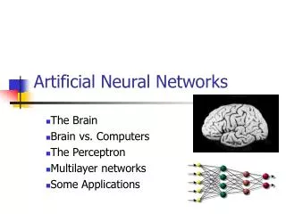
INTRODUCTIONBiological Motivation • Human brain is a densely interconnected network of approximately 1011 neurons, each connected to, on average, 104 others. • Neuron activity is excited or inhibited through connections to other neurons. • The fastest neuron switching times are known to be on the order of 10-3 sec.
The cell itself includes a nucleus (at the center). • To the right of cell 2, the dendrites provide input signals to the cell. • To the right of cell 1, the axon sends output signals to cell 2 via the axon terminals. These axon terminals merge with the dendrites of cell 2.
Portion of a network: two interconnected cells. • Signals can be transmitted unchanged or they can be altered by synapses. A synapse is able to increase or decrease the strength of the connection from the neuron to neuron and cause excitation or inhibition of a subsequence neuron. This is where information is stored. • The information processing abilities of biological neural systems must follow from highly parallel processes operating on representations that are distributed over many neurons. One motivation for ANN is to capture this kind of highly parallel computation based on distributed representations.
2. NEURAL NETWORK REPRESENTATION • An ANN is composed of processing elements called or perceptrons, organized in different ways to form the network’s structure. Processing Elements • An ANN consists of perceptrons. Each of the perceptrons receives inputs, processes inputs and delivers a single output. The input can be raw input data or the output of other perceptrons. The output can be the final result (e.g. 1 means yes, 0 means no) or it can be inputs to other perceptrons.
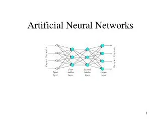
The network • Each ANN is composed of a collection of perceptrons grouped in layers. A typical structure is shown in Fig.2. Note the three layers: input, intermediate (called the hidden layer) and output. Several hidden layers can be placed between the input and output layers.
Appropriate Problems for Neural Network • ANN learning is well-suited to problems in which the training data corresponds to noisy, complex sensor data. It is also applicable to problems for which more symbolic representations are used. • The backpropagation (BP) algorithm is the most commonly used ANN learning technique. It is appropriate for problems with the characteristics: • Input is high-dimensional discrete or real-valued (e.g. raw sensor input) • Output is discrete or real valued • Output is a vector of values • Possibly noisy data • Long training times accepted • Fast evaluation of the learned function required. • Not important for humans to understand the weights • Examples: • Speech phoneme recognition • Image classification • Financial prediction
3. PERCEPTRONS • A perceptron takes a vector of real-valued inputs, calculates a linear combination of these inputs, then outputs • a 1 if the result is greater than some threshold • –1 otherwise. • Given real-valued inputs x1 through xn, the output o(x1, …, xn) computed by the perceptron is o(x1, …, xn) = 1 if w0 + w1x1 + … + wnxn > 0 -1 otherwise where wi is a real-valued constant, or weight. • Notice the quantify (-w0) is a threshold that the weighted combination of inputs w1x1 + … + wnxn must surpass in order for perceptron to output a 1.
To simplify notation, we imagine an additional constant input x0 = 1, allowing us to write the above inequality as n i=0 wixi >0 • Learning a perceptron involves choosing values for the weights w0, w1,…, wn. Figure 3. A perceptron
Representation Power of Perceptrons • We can view the perceptron as representing a hyperplane decision surface in the n-dimensional space of instances (i.e. points). The perceptron outputs a 1 for instances lying on one side of the hyperplane and outputs a –1 for instances lying on the other side, as in Figure 4. The equation for this decision hyperplane is Some sets of positive and negative examples cannot be separated by any hyperplane. Those that can be separated are called linearly separated set of examples. Figure 4. Decision surface
A single perceptron can be used to represent many boolean functions.AND function : Decision hyperplane : w0 + w1 x1 + w2 x2 = 0 -0.8 + 0.5 x1 + 0.5 x2 = 0
OR function • The two-input perceptron can implement the OR function when we set the weights: w0 = -0.3, w1 = w2 = 0.5 Decision hyperplane : w0 + w1 x1 + w2 x2 = 0 -0.3 + 0.5 x1 + 0.5 x2 = 0
XOR function : It’s impossible to implement the XOR function by a single perception. A two-layer network of perceptrons can represent XOR function. Refer to this equation,
Perceptron training rule • Although we are interested in learning networks of many interconnected units, let us begin by understanding how to learn the weights for a single perceptron. • Here learning is to determine a weight vector that causes the perceptron to produce the correct +1 or –1 for each of the given training examples. • Several algorithms are known to solve this learning problem. Here we consider two: the perceptron rule and the delta rule.
One way to learn an acceptable weight vector is to begin with random weights, then iteratively apply the perceptron to each training example, modifying the perceptron weights whenever it misclassifies an example. This process is repeated, iterating through the training examples as many as times needed until the perceptron classifies all training examples correctly. • Weights are modified at each step according to the perceptron training rule, which revises the weight wi associated with input xi according to the rule. wiwi + wi where wi = (t – o) xi • Here: t is target output value for the current training example o is perceptron output is small constant (e.g., 0.1) called learning rate
Perceptron training rule (cont.) • The role of the learning rate is to moderate the degree to which weights are changed at each step. It is usually set to some small value (e.g. 0.1) and is sometimes made to decrease as the number of weight-tuning iterations increases. • We can prove that the algorithm will converge • If training data is linearly separable • and sufficiently small. • If the data is not linearly separable, convergence is not assured.
Gradient Descent and the Delta Rule • Although the perceptron rule finds a successful weight vector when the training examples are linearly separable, it can fail to converge if the examples are not linearly separatable. A second training rule, called the delta rule, is designed to overcome this difficulty. • The key idea of delta rule: to use gradient descent to search the space of possible weight vector to find the weights that best fit the training examples. This rule is important because it provides the basis for the backpropagration algorithm, which can learn networks with many interconnected units. • The delta training rule: considering the task of training an unthresholded perceptron, that is a linear unit, for which the output o is given by: o = w0+ w1x1 + ··· + wnxn (1) • Thus, a linear unit corresponds to the first stage of a perceptron, without the threhold.
In order to derive a weight learning rule for linear units, let specify a measure for the training error of a weight vector, relative to the training examples. The Training Error can be computed as the following squared error (2) where D is set of training examples, td is the target output for the training example d and od is the output of the linear unit for the training example d. Here we characterize E as a function of weight vector because the linear unit output O depends on this weight vector.
Hypothesis Space • To understand the gradient descent algorithm, it is helpful to visualize the entire space of possible weight vectors and their associated E values, as illustrated in Figure 5. • Here the axes wo,w1 represents possible values for the two weights of a simple linear unit. The wo,w1 plane represents the entire hypothesis space. • The vertical axis indicates the error E relative to some fixed set of training examples. The error surface shown in the figure summarizes the desirability of every weight vector in the hypothesis space. • For linear units, this error surface must be parabolic with a single global minimum. And we desire a weight vector with this minimum.
Figure 5. The error surface How can we calculate the direction of steepest descent along the error surface? This direction can be found by computing the derivative of E w.r.t. each component of the vector w.
Derivation of the Gradient Descent Rule • This vector derivative is called the gradient of E with respect to the vector <w0,…,wn>, written E . (3) Notice E is itself a vector, whose components are the partial derivatives of E with respect to each of the wi. When interpreted as a vector in weight space, the gradient specifies the direction that produces the steepest increase in E. The negative of this vector therefore gives the direction of steepest decrease. Since the gradient specifies the direction of steepest increase of E, the training rule for gradient descent is ww + w where (4)
Here is a positive constant called the learning rate, which determines the step size in the gradient descent search. The negative sign is present because we want to move the weight vector in the direction that decreases E. This training rule can also be written in its component form wiwi + wi where (5) which makes it clear that steepest descent is achieved by altering each component wi of weight vector in proportion to E/wi. The vector of E/wi derivatives that form the gradient can be obtained by differentiating E from Equation (2), as
(6) where xid denotes the single input component xi for the training example d. We now have an equation that gives E/wi in terms of the linear unit inputs xid, output od and the target value td associated with the training example. Substituting Equation (6) into Equation (5) yields the weight update rule for gradient descent.
(7) • The gradient descent algorithm for training linear units is as follows: Pick an initial random weight vector. Apply the linear unit to all training examples, them compute wi for each weight according to Equation (7). Update each weight wi by adding wi , them repeat the process. The algorithm is given in Figure 6. • Because the error surface contains only a single global minimum, this algorithm will converge to a weight vector with minimum error, regardless of whether the training examples are linearly separable, given a sufficiently small is used. • If is too large, the gradient descent search runs the risk of overstepping the minimum in the error surface rather than settling into it. For this reason, one common modification to the algorithm is to gradually reduce the value of as the number of gradient descent steps grows.
Figure 6. Gradient Descent algorithm for training a linear unit.
Stochastic Approximation to Gradient Descent • The key practical difficulties in applying gradient descent are: • Converging to a local minimum can sometimes be quite slow (i.e., it can require many thousands of steps). • If there are multiple local minima in the error surface, then there is no guarantee that the procedure will find the global minimum. • One common variation on gradient descent intended to alleviate these difficulties is called incremental gradient descent (or stochastic gradient descent). The key differences between standard gradient descent and stochastic gradient descent are: • In standard gradient descent, the error is summed over all examples before upgrading weights, whereas in stochastic gradient descent weights are updated upon examining eachtraining example. • The modified training rule is like the training example we update the weight according to wi = (t – o) xi (10)
Summing over multiple examples in standard gradient descent requires more computation per weight update step. On the other hand, because it uses the true gradient, standard gradient descent is often used with a larger step size per weight update than stochastic gradient descent.
Stochastic gradient descent (i.e. incremental mode) can sometimes avoid falling into local minima because it uses the various gradient of E rather than overall gradient of E to guide its search. • Both stochastic and standard gradient descent methods are commonly used in practice. Summary • Perceptron training rule • Perfectly classifies training data • Converge, provided the training examples are linearly separable • Delta Rule using gradient descent • Converge asymptotically to minimum error hypothesis • Converge regardless of whether training data are linearly separable
3. MULTILAYER NETWORKS AND THE BACKPROPOGATION ALGORITHM • Single perceptrons can only express linear decision surfaces. In contrast, the kind of multilayer networks learned by the backpropagation algorithm are capaple of expressing a rich variety of nonlinear decision surfaces. • This section discusses how to learn such multilayer networks using a gradient descent algorithm similar to that discussed in the previous section. A Differentiable Threshold Unit • What type of unit as the basis for multilayer networks ? Perceptron : not differentiable -> can’t use gradient descent Linear Unit : multi-layers of linear units -> still produce only linear function Sigmoid Unit : smoothed, differentiable threshold function
Like the perceptron, the sigmoid unit first computes a linear combination of its inputs, then applies a threshold to the result. In the case of sigmoid unit, however, the threshold output is a continuous function of its input. • The sigmoid function (x) is also called the logistic function. • Interesting property: Output ranges between 0 and 1, increasing monotonically with its input. We can derive gradient decent rules to train One sigmoid unit Multilayer networks of sigmoid units Backpropagation
The Backpropagation (BP)Algorithm • The BP algorithm learns the weights for a multilayer network, given a network with a fixed set of units and interconnections. It employs a gradient descent to attempt to minimize the squared error between the network output values and the target values for these outputs. • Because we are considering networks with multiple output units rather than single units as before, we begin by redefining E to sum the errors over all of the network output units • E(w) = ½ (tkd – okd)2 (13) d D koutputs where outputs is the set of output units in the network, and tkd and okd are the target and output values associated with the kth output unit and training example d.
The Backpropagation Algorithm (cont.) • The BP algorithm is presented in Figure 8. The algorithm applies to layered feedforward networks containing 2 layers of sigmoid units, with units at each layer connected to all units from the preceding layer. • This is an incremental gradient descent version of Backpropagation. • The notation is as follows: • xij denotes the input from node i to unit j, and wij denotes the corresponding weight. • n denotes the error term associated with unit n. It plays a role analogous to the quantity (t – o) in our earlier discussion of the delta training rule.
In the BP algorithm, step1 propagates the input forward through the network. And the steps 2, 3 and 4 propagates the errors backward through the network. • The main loop of BP repeatedly iterates over the training examples. For each training example, it applies the ANN to the example, calculates the error of the network output for this example, computes the gradient with respect to the error on the example, then updates all weights in the network. This gradient descent step is iterated until ANN performs acceptably well. • A variety of termination conditions can be used to halt the procedure. • One may choose to halt after a fixed number of iterations through the loop, or • once the error on the training examples falls below some threshold, or • once the error on a separate validation set of examples meets some criteria.
Adding Momentum • Because BP is a widely used algorithm, many variations have been developed. The most common is to alter the weight-update rule in Step 4 in the algorithm by making the weight update on the nth iteration depend partially on the update that occurred during the (n -1)th iteration, as follows: • Here wi,j(n) is the weight update performed during the n-th iteration through the main loop of the algorithm. • - n-th iteration update depend on (n-1)th iteration • - : constant between 0 and 1 is called the momentum. • Role of momentum term: • - keep the ball rolling through small local minima in the error surface. • - Gradually increase the step size of the search in regions where the gradient is unchanging, thereby speeding convergence.
REMARKS ON THE BACKPROPAGATION ALGORITHM • Convergence and Local Minima • Gradient descent to some local minimum • Perhaps not global minimum... • Heuristics to alleviate the problem of local minima • Add momentum • Use stochastic gradient descent rather than true gradient descent. • Train multiple nets with different initial weights using the same data.
Expressive Capabilities of ANNs • Boolean functions: • Every boolean function can be represented by network with two layers of units where the number of hidden units required grows exponentially. • Continuous functions: • Every bounded continuous function can be approximated with arbitrarily small error, by network with two layers of units [Cybenko 1989; Hornik et al. 1989] • Arbitrary functions: • Any function can be approximated to arbitrary accuracy by a network with three layers of units [Cybenko 1988].
Hidden layer representations • Hidden layer representations • This 8x3x8 network was trained to learn the identity function. • 8 training examples are used. • After 5000 training iterations, the three hidden unit values encode the eight distinct inputs using the encoding shown on the right.
Learning the 8x3x8 network Most of the interesting weight changes occurred during the first 2500 iterations. Figure 10.a The plot shows the sum of squared errors for each of the eight output units as the number of iterations increases. The sum of square errors for each output decreases as the procedure proceeds, more quickly for some output units and less quickly for others.
Figure 10.b Learning the 8 3 8 network. The plot shows the evolving hidden layer representation for the input string “010000000”. The network passes through a number of different encodings before converging to the final encoding.
Generalization, Overfitting and Stopping Criterion • Termination condition • Until the error E falls below some predetermined threshold • This is a poor strategy • Overfitting problem • Backpropagation is susceptible to overfitting the training examples at the cost of decreasing generalization accuracy over other unseen examples. • To see the danger of minimizing the error over the training data, consider how the error E varies with the number of weight iteration.
The generalization accuracy measured over the training examples first decreases, then increases, even as the error over training examples continues to decrease. This occurs because the weights are being tuned to fit idiosyncrasies of the training examples that are not representative of the general distribution of examples.
Techniques to overcome overfitting problem • Weight decay : Decrease each weight by some small factor during each iteration. The motivation for this approach is to keep weight values small. • Cross-validation: a set of validation data in addition to the training data. The algorithm monitors the error w.r.t. this validation data while using the training set to drive the gradient descent search. • How many weight-tuning iterations should the algorithm perform? It should use the number of iterations that produces the lowest error over the validation set. • Two copies of the weights are kept: one copy for training and a separate copy of the best weights thus far, measured by their error over the validation set. • Once the trained weights reach a higher error over the validation set than the stored weights, training is terminated and the stored weights are returned.
NEURAL NETWORK APPLICATION DEVELOPMENT The development process for an ANN application has eight steps. • Step 1: (Data collection) The data to be used for the training and testing of the network are collected. Important considerations are that the particular problem is amenable to neural network solution and that adequate data exist and can be obtained. • Step 2: (Training and testing data separation) Trainning data must be identified, and a plan must be made for testing the performance of the network. The available data are divided into training and testing data sets. For a moderately sized data set, 80% of the data are randomly selected for training, 10% for testing, and 10% secondary testing. • Step 3: (Network architecture) A network architecture and a learning method are selected. Important considerations are the exact number of perceptrons and the number of layers.
Step 4: (Parameter tuning and weight initialization) There are parameters for tuning the network to the desired learning performance level. Part of this step is initialization of the network weights and parameters, followed by modification of the parameters as training performance feedback is received. • Often, the initial values are important in determining the effectiveness and length of training. • Step 5: (Data transformation) Transforms the application data into the type and format required by the ANN. • Step 6: (Training) Training is conducted iteratively by presenting input and desired or known output data to the ANN. The ANN computes the outputs and adjusts the weights until the computed outputs are within an acceptable tolerance of the known outputs for the input cases.
Step 7: (Testing) Once the training has been completed, it is necessary to test the network. • The testing examines the performance of the network using the derived weights by measuring the ability of the network to classify the testing data correctly. • Black-box testing (comparing test results to historical results) is the primary approach for verifying that inputs produce the appropriate outputs. • Step 8: (Implementation) Now a stable set of weights are obtained. • Now the network can reproduce the desired output given inputs like those in the training set. • The network is ready to use as a stand-alone system or as part of another software system where new input data will be presented to it and its output will be a recommended decision.
BENEFITS AND LIMITATIONS OF NEURAL NETWORKS 6.1 Benefits of ANNs • Usefulness for pattern recognition, classification, generalization, abstraction and interpretation of imcomplete and noisy inputs. (e.g. handwriting recognition, image recognition, voice and speech recognition, weather forecasing). • Providing some human characteristics to problem solving that are difficult to simulate using the logical, analytical techniques of expert systems and standard software technologies. (e.g. financial applications). • Ability to solve new kinds of problems. ANNs are particularly effective at solving problems whose solutions are difficult, if not impossible, to define. This opened up a new range of decision support applications formerly either difficult or impossible to computerize.
Robustness. ANNs tend to be more robust than their conventional counterparts. They have the ability to cope with imcomplete or fuzzy data. ANNs can be very tolerant of faults if properly implemented. • Fast processing speed. Because they consist of a large number of massively interconnected processing units, all operating in parallel on the same problem, ANNs can potentially operate at considerable speed (when implemented on parallel processors). • Flexibility and ease of maintenaince. ANNs are very flexible in adapting their behavior to new and changing environments. They are also easier to maintain, with some having the ability to learn from experience to improve their own performance. 6.2 Limitations of ANNs • ANNs do not produce an explicit model even though new cases can be fed into it and new results obtained. • ANNs lack explanation capabilities. Justifications for results is difficults to obtain because the connection weights usually do not have obvious interpretaions.
