Download
1 / 11
110 likes | 165 Vues
Explore Bode plots for first and second-order systems, learn about Butterworth and Chebyshev filters, frequency transformations, and filter design strategies. Discover how to approximate frequency responses and design efficient filters in MATLAB.

E N D
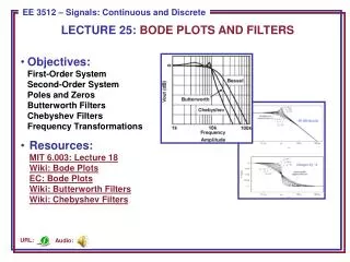
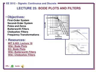
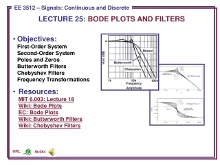
LECTURE 25: BODE PLOTS AND FILTERS • Objectives:First-Order SystemSecond-Order SystemPoles and ZerosButterworth FiltersChebyshev FiltersFrequency Transformations • Resources:MIT 6.003: Lecture 18Wiki: Bode PlotsEC: Bode PlotsWiki: Butterworth FiltersWiki: Chebyshev Filters Audio: URL:
First-Order System Revisited • Recall the transfer functionfor a 1st-order system: • The frequency response of thissystem is:
Bode Plot • Asymptotic approximation tothe actual frequency response. • Plotted on a log-log scale. • Allows approximation of thefrequency response usingstraight lines: • Note that: 20 dB/decade Changes by /2
Second-Order System • The transfer function of a 2nd-order system: • The frequency response of thissystem can be modeled as: • When : 40 dB/decade Changes by
Example: Poles and Zeroes • Transfer function: • The critical frequenciesare = 2 (zero), 10 (pole),and 50 (pole). • MATLAB (exact resp.): • w = logspace(-1,3,300); • s = j*w; • H = 1000*(s+2)./(s+10)./(s+50); • magdB = 20*log10(abs(H)); • phase = angle(H)*180/pi; • MATLAB (Bode): • num = [1000 2000]; • den = conv([1 1o], [1 50]); • bode(num, den); • Bode plots are useful as ananalytic tool.
Causal Filters • Recall that the ideal lowpass filter is a noncausal filter and henceunrealizable. • The filter design problem thenbecomes an optimization problemin which we try to best meet theuser’s requirements with a filter thatcan be implemented with the least number of components. • This is equivalent to trying to minimize the number of coefficients in the (Laplace transform) transfer function. It is also comparable to minimizing the order of the filter. • Typically the numerator order is less than or equal to the denominator order, so, building on the concept of a Bode plot, we can relate the maximum amount of attenuation desired to the order of the denominator. • There are often no “perfect” solutions. Users must tradeoff design constraints such as passband smoothness, stopband attenuation and linearity in phase. • Computer-aided design programs, including MATLAB, are able to design filters once the user adequately specifies the constraints. We will explore two interesting analytic solutions: Butterworth and Chebyshev filters.
Butterworth Filters • Butterworth filters are maximally flat in the passband. Their distinguishing characteristic isthat the poles are arranged on a semi-circle ofradius c in the left-half plane. • The filter function is an all-pole filter that exploitsthe properties of Butterworth polynomials. • Examples: • Frequency Response: • Design strategy: select the cutofffrequency and the amount of stopband attenuation, thencompute the order of the filter.
Chebyshev Filters • Chebyshev filter, based on Chebyshev polynomials, allows ripple in the passband to achieve greater attenuation. This implies a lower filter order at the expense of smoothness of the frequency response in the passband. • Prototype: • where: • and is chosen based on the amount of passband ripple that can be tolerated. • Filter design theory is basedlargely on the mathematicalproperties of polynomials. • An third type of filter, the elliptical filter, attempts toallow ripple in both bands.
Frequency Transformations • There are two general approaches tofilter design: • Direct optimization of the desired frequency response, typicallyusing software like MATLAB. • Design a “normalized” lowpassfilter and then transform it to another lowpass, highpass orbandpass filter. • The latter approach can be achieved by using these simple frequency transformations: • This latter approach is popularbecause it leverages our knowledgeof the properties of lowpass filters.
Summary • Analyzed the frequency response of a first and second-order system. • Demonstrated how this can be approximated using Bode plots. • Demonstrated that the Bode plot can be used to construct the frequency and phase responses of complex systems. • Introduced Butterworth and Chebyshev lowpass filters. • Described how lowpass filters can be converted to bandpass and highpass filters using a frequency transformation.