Binomial heaps, Fibonacci heaps, and applications
370 likes | 540 Vues
Binomial heaps, Fibonacci heaps, and applications. Dijkstra’s shortest path algorithm. Let G = (V,E) be a weighted (weights are non-negative) undirected graph, let s V. Want to find the distance (length of the shortest path), d(s,v) from s to every other vertex. 3. 3. s. 2. 1. 3. 2.

Binomial heaps, Fibonacci heaps, and applications
E N D
Presentation Transcript
Dijkstra’s shortest path algorithm Let G = (V,E) be a weighted (weights are non-negative) undirected graph, let s V. Want to find the distance (length of the shortest path), d(s,v) from s to every other vertex. 3 3 s 2 1 3 2
How many times we do these operations in Dijkstra’s algorithm ? • Insert(x,Q) • min(Q) • Deletemin(Q) • Decrease-key(x,Q,Δ): Can simulate by Delete(x,Q), insert(x-Δ,Q) Overall running time O(nlog n + m log n) n = |V| n n m = |E|
Binomial trees B0 B1 Bi B(i-1) B(i-1)
Binomial trees Bi . . . . . . B0 B(i-1) B(i-2) B1
Properties of binomial trees 1) | Bk | = 2k 2) degree(root(Bk))= k 3) depth(Bk)= k ==> The degree and depth of a binomial tree with at most n nodes is at most log(n). Define the rank of Bk to be k
5 1 5 2 5 5 6 6 8 9 10 Binomial heaps (def) A collection of binomial trees at most one of every rank. Items at the nodes, heap ordered. Possible rep: Doubly link roots and children of every node. Parent pointers needed for delete.
5 1 5 5 2 6 6 4 10 6 8 9 9 11 9 10 Binomial heaps (operations) Operations are defined via a basic operation, called linking, of binomial trees: Produce a Bk from two Bk-1, keep heap order.
Binomial heaps (ops cont.) Basic operation is meld(h1,h2): Like addition of binary numbers. B5 B4 B2 B1 h1: B4 B3 B1 B0 + h2: B4 B3 B0 B5 B4 B2
Binomial heaps (ops cont.) Findmin(h): obvious Insert(x,h) : meld a new heap with a single B0 containing x, with h deletemin(h) : Chop off the minimal root. Meld the subtrees with h. Update minimum pointer if needed. delete(x,h) : Bubble up and continue like delete-min decrease-key(x,h,) : Bubble up, update min ptr if needed All operations take O(log n) time on the worst case, except find-min(h) that takes O(1) time.
Amortized analysis We are interested in the worst case running time of a sequenceof operations. Example: binary counter single operation -- increment 00000 00001 00010 00011 00100 00101
Amortized analysis (Cont.) On the worst case increment takes O(k). k = #digits What is the complexity of a sequence of increments (on the worst case) ? Define a potential of the counter: (c) = ? Amortized(increment) = actual(increment) +
+ Amortized analysis (Cont.) Amortized(increment1) = actual(increment1) + 1-0 Amortized(increment2) = actual(increment2) + 2-1 … … Amortized(incrementn) = actual(incrementn) + n-(n-1) iAmortized(incrementi) = iactual(incrementi) + n-0 iAmortized(incrementi) iactual(incrementi) if n-0 0
Amortized analysis (Cont.) Define a potential of the counter: (c) = #(ones) Amortized(increment) = actual(increment) + Amortized(increment) = 1+ #(1 => 0) + 1 - #(1 => 0) = O(1) ==> Sequence of n increments takes O(n) time
Binomial heaps - amortized ana. (collection of heaps) = #(trees) Amortized cost of insert O(1) What if other operations are also introduced? Amortized cost of other operations still O(log n)
Binomial heaps + lazy meld Allow more than one tree of each rank. • Meld (h1,h2) : • Concatenate the lists of binomial trees. • Update the minimum pointer to be the smaller of the minimums O(1) worst case and amortized.
Binomial heaps + lazy meld As long as we do not do a delete-min our heaps are just doubly linked lists: 9 11 4 6 9 5 Delete-min : Chop off the minimum root, add its children to the list of trees. Successive linking: Traverse the forest keep linking trees of the same rank, maintain a pointer to the minimum root.
Binomial heaps + lazy meld Possible implementation of delete-min is using an array indexed by rank to keep at most one binomial tree of each rank that we already traversed. Once we encounter a second tree of some rank we link them and keep linking until we do not have two trees of the same rank. We record the resulting tree in the array Amortized(delete-min) = = (#links + max-rank) – (#links – max-rank) = O(log(n))
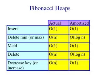
What do we have so far? • FindMin – O(1) worst case • Meld – O(1) worst case • Insert – O(1) worst case • DeleteMin – O(log n) amortized • DecreaseKey – O(log n) amortized
Fibonacci heaps (Fredman & Tarjan 84) Want to do decrease-key(x,h,) faster than delete+insert. Ideally in O(1) time. Why ?
Dijkstra’s shortest path algorithm Let G = (V,E) be a weighted (weights are non-negative) undirected graph, let s V. Want to find the distance (length of the shortest path), d(s,v) from s to every other vertex. 3 3 s 2 1 3 2
How many times we do these operations ? • Insert(x,Q) • min(Q) • Deletemin(Q) • Decrease-key(x,Q,Δ): This time: O(n log n + m) n = |V| n n m = |E|
Application #2 : Prim’s algorithm for Minimum Spanning Tree Start with T a singleton vertex. Grow a tree by repeating the following step: Add the minimum cost edge connecting a vertex in T to a vertex out of T.
Application #2 : Prim’s algorithm for Minimum Spanning Tree Maintain the vertices out of T but adjacent to T in a heap. The key of a vertex v is the weight of the lightest edge (v,w) where w is in the tree. Iteration: Do a delete-min. Let v be the minimum vertex and (v,w) the lightest edge as above. Add (v,w) to T. For each edge (v,u) where uT, if key(u) = insert u into the heap with key(u) = w(v,u) if w(v,u) < key(u) decrease the key of u to be w(v,u). With regular heaps O(m log(n)). With F-heaps O(n log(n) + m).
Suggested implementation for decrease-key(x,h,): If x with its new key is smaller than its parent, cut the subtree rooted at x and add it to the forest. Update the minimum pointer if necessary.
5 5 2 5 3 1 5 2 5 5 5 5 10 6 9 6 8 8 6 9 6 10 DecreaseKey(3,h,2)
Decrease-key (cont.) Does it work ? Obs1: Trees need not be binomial trees any more.. Do we need the trees to be binomial ? Where have we used it ? In the analysis of delete-min we used the fact that at most log(n) new trees are added to the forest. This was obvious since trees were binomial and contained at most n nodes.
2 9 5 3 6 5 6 Decrease-key (cont.) Such trees are now legitimate. So our analysis breaks down.
Fibonacci heaps (cont.) We shall allow non-binomial trees, but will keep the degrees logarithmic in the number of nodes. Rank of a tree = degree of the root. Delete-min: do successive linking of trees of the same rank and update the minimum pointer as before. Insert and meld also work as before.
Fibonacci heaps (cont.) Decrease-key (x,h,): indeed cuts the subtree rooted by x if necessary as we showed. in addition we maintain a mark bit for every node. When we cut the subtree rooted by x we check the mark bit of p(x). If it is set then we cut p(x) too. We continue this way until either we reach an unmarked node in which case we mark it, or we reach the root. This mechanism is called cascading cuts.
9 5 7 4 2 20 16 6 14 8 11 12 15 2 4 20 5 8 11 9 6 14 10 16 12 15
Fibonacci heaps (delete) Delete(x,h) : Cut the subtree rooted at x and then proceed with cascading cuts as for decrease key. Chop off x from being the root of its subtree and add the subtrees rooted by its children to the forest If x is the minimum node do successive linking
Fibonacci heaps (analysis) Want everything to be O(1) time except for delete and delete-min. ==> cascading cuts should pay for themselves (collection of heaps) = #(trees) + 2#(marked nodes) Actual(decrease-key) = O(1) + #(cascading cuts) (decrease-key) = O(1) - #(cascading cuts) ==> amortized(decrease-key) = O(1) !
Fibonacci heaps (analysis) What about delete and delete-min ? Cascading cuts and successive linking will pay for themselves. The only question is what is the maximum degree of a node ? How many trees are being added into the forest when we chop off a root ?
x Proof: When the i-th node was linked it must have had at least i-1 children. Since then it could have lost at most one. Fibonacci heaps (analysis) Lemma 1 : Let x be any node in an F-heap. Arrange the children of x in the order they were linked to x, from earliest to latest. Then the i-th child of x has rank at least i-2. 2 1
x Fibonacci heaps (analysis) Corollary1 : A node x of rank k in a F-heap has at least k descendants, where = (1 + 5)/2 is the golden ratio. Proof: Let sk be the minimum number of descendants of a node of rank k in a F-heap. By Lemma 1 sk i=0si + 2 k-2 s0=1, s1= 2
Fibonacci heaps (analysis) Proof (cont): Fibonnaci numbers satisfy Fk+2 = i=2Fi + 2, for k 2, and F2=1 so by induction sk Fk+2 It is well known that Fk+2 k k It follows that the maximum degree k in a F-heap with n nodes is such that k n so k log(n) / log() = 1.4404 log(n)