Download
1 / 64
640 likes | 675 Vues
Explore the concepts, measurements, and applications of transverse emittances in particle beams, clarifying terminology and units. Learn how emittance impacts beam focus and design of accelerators. Understand normalized and RMS emittance for accurate beam analysis.

E N D
Measuring and Analyzing Transverse Emittances of Charged Particle Beams Martin P. Stockli and many collogues at SNS and other Accelerator Labs BIW’06 Fermi National Accelerator Laboratory Batavia, IL, May 1, 2006
Outline: • Concepts and Definitions • Applications • The Emittance Ellipse • Dilemmas • Measuring Emittance Distributions (Destructive) • Nondestructive Measurements of the Emittance Ellipse • Analysis of emittance Ellipse • Analysis of Emittance Distributions • Conclusions
The Emittance p The emittance is the 6-dimensional hypervolume in the phase space x,y,z,px,py,pz that is occupied by a number of beam particles. The coordinates are normally referenced with respect to the center, by zeroing the first moments: y (x0,y0,z0) x z If the axial motion does not couple to the transverse motions, the hypervolume can be separated into the 2-dimensional longitudinal emittance, which describes the beam current profile as a function of time, and the transverse emittance which describes the beam current as a function of transverse position. The transverse emittance is the 4-dimensional, occupied hypervolume in the phase space x,y,px,py: If transverse motions are not coupled, the emittance can be separated into its components, which form 2-dimensional areas in {x,px} and {y,py}: with form-factor 2
Emittance in Trace-Space: For pz invariant along the beam axis, p can be factored out, yielding the transverse emittance in the trace space x,y, x=dx/dz, and y=dy/dz. If transverse motions are not coupled, the emittance can be separated into its components, which form the 2-dimensional areas {x,x} and {y,y}: All these terms are normally called “Emittance”. However, rigorous authors call them either “Volume Emittance” or “Area Emittance”. Most then go on to introduce the “Emittance” as the semi-axis-product of an hyper-ellipsoid with the same area or volume: Confusion can be avoided by stating whether the quoted emittance value is a volume, an area, or a semi-axis-product!
Units of Emittances in the Trace-Space Emittances have the dimension of (lengthangle)n. Common are mm·mrad, cm·mrad, and m·rad However, the radian angle is a dimensionless ratio, and therefore some people use m, mm, and m (= mm·mrad). For semi-axis-products it is common to write mm·mrad, cm·mrad, or m·rad The is supposed “to assure the reader that the has the has been factored out of the phase space area (Sanders, 1990).” However, if the was factored out, it was factored out in the definition. The in the unit has no clear meaning. It is neither a real unit, nor a true multiplier. It is a one-of-a-kind object that has no precedent in the physics literature! It has created as much confusion as it intended to eliminate. A trend has started to omit the in the unit. Confusion can be avoided by stating whether the quoted emittance value is a volume, an area, or a semi-axis-product! Unless otherwise stated, semi-axis-products will be quoted throughout this presentation!
Normalized Emittances x2 x1 vT vT As the particles are accelerated from vz1 to vz2, the trace angles narrow, causing the emittance to shrink. vz1 vz2 The emittance can be normalized by multiplying the emittance with the dimensionless particle-velocity to speed-of-light ratio: with and with or The normalized emittance stays roughly the same throughout most parts of most accelerators!
The RMS Emittance Emittance volumes or areas that contain all particles are of limited merit because they are very large and dominated by a very few particles of questionable character. The volume of an entire Gaussian distribution is infinite. This problem can be reduced by quoting the emittance volume of a certain fraction of the beam, e.g. 90%, yielding E90% or A 90% . The problem is resolved with the rms emittance that averages over all particles with a weight given by the particles distance from the “center”: , e.g.: , with , , and , This is the semi-axis-product of an ellipse. For a Gaussian distribution, the ellipse contains 39% of the beam. (E90% = 4.6Erms) For a finite current , the rms-emittance is finite. There is no absolute need to threshold the data, but tresholded rms-emittances are common, e.g. E rms,90%. Unfortunately many authors fail to be specific!
What is it all good for? • According to Liouville’s theorem, emittances are conserved if the particles are subjected only to conservative forces, such as time-invariant electric and magnetic fields. Therefore the emittance allows for predicting the downstream beam transport, the beam’s focusability, the losses in downstream restricted beam line apertures, etc. It is invaluable for designing accelerators and beam lines! • Some non-conservative forces, such as collisions, scattering, and fluctuations of electric or magnetic fields, increase the emittance. • Other non-conservative forces, such as E-M radiation, decrease the emittance. • The emittance is conserved under space charge as long as the forces are caused by the charged particle cloud, rather than by individual particles. Due to the nature of the beam formation in ion sources and/or the collimation in the extractor- and other apertures, emittances are normally of elliptical shape. Beams collimated by rectangular wave guides (in dipole magnets) or by straight slits can exhibit rectangular shapes. In this presentation we will focus on elliptical emittances.
The Emittance ellipse While the area is constant, the emittance ellipse shape and orientation changes. It is described by: beam waist beam envelope z x x x x x x x x
The Ellipse and the Twiss parameter: diverging beam: <0 waist or lens: =0 converging beam >0 x >0 by definition [mm/mrad] 0<= constant [mmmrad] a x [mrad/mm] b Divergence: Beam radius: Orientation: Aspect ratio:
The Transformation of Ellipses: The transfer matrix is normally used to calculate individual particle rays: with e.g.: or Similarly, the ellipse equation can be written as: with Which allows to calculate the beam envelope as:
Real emittances: SNS LEBT (65 keV) SNS MEBT (2.5 MeV) ~70 mrad ~15 mrad • Angular spread shrinks as as beam is accelerated. • Non linear forces, such as lens aberrations and space charge, often cause low-energy emittances to be S-shaped. • Particles far from the central ellipse are preferentially lost in the RFQ. Ellipses are good approximations for high energy beams.
Emittance Dilemmas: Focused by linear forces Focused by non-linear forces Initial beam • Liouville’s theorem applies to the area that is conserved. • Elliptical approximations do not work very well at low beam energies. To calculate losses and acceptances one has to fit the smallest ellipse that encloses the desired beam fraction. These ellipses are not conserved. • RMS emittances are only conserved for systems with linear forces (elliptical emittances). Despite, they are normally a useful figure of merit!
A Pedestrian Emittance Measurement: x d2 x • The x% emittance can be approximately determined with 2 pairs of slits separated by distance L in a drift space: • Open fully one of the pair of slits while narrowing the other pair. • Maximize beam transmission through the narrow set of slits. • Set both collimating slits to cut (1-x)/4 of the beam. Repeat 2 & 3 as needed. • Set the corresponding slits of the other set to each remove another (1-x)/4 of the beam. • Read the (1+x)/2 % beam waist diameter dW and the (1+x)/2 % downstream beam diameter d2. Ex%dW(d2-dW)/(4L). x x dW
Measuring Emittances Measuring the 4-dimensional emittance requires 4 pairs of slits • First 2 pairs define the geometrical position x, x, y, y • Distance L downstream a 2nd set defines the tangent of the traces x’, x’, y’, y’ • The Faraday cup measures only the current passing through all slits! This is the only method to measure with infinite resolution all detailed ion beam information, including coupling between x and y motions.
Measuring Emittances The measured current signal • Problems: • The measured current signal c(x,y,x’,y’) is very small: c Itot/104 • Requires Nx·Ny·Nx’·Ny’ measurements, e.g. 108 for 100 positions per scan • Takes forever or longer!
Pepper Pot Emittance Probe Uses a pepper-pot plate to form many small beamlets from the beam. Holes ~0.05mm, 2-3 mm apart. A truly 4 dimensional, single shot measurement, but with limited resolution. Samples only ~0.1% of the beam, yielding tiny signals. Traditionally used screens and/or photographic paper. Electronic readout possible with CCD camera or high density wire screens. For axial-symmetric beams the full emittance to be calculated as • = (RD/2z)(Dz/d – Sz/S)(1-(S/R)2)-1/2 (J.G. Wang et al.) With D, Dz hole and image diameter S, Sz distance from beam center Z distance between pepper pot and screen R full beam radius at pepper pot
The GSI Pepper Pot, State of the Art: 15x15 0.1 mm holes, 2.5 mm apart Pepper-pot plate continues to improve Alumina (Al2O3) screen Separation adjustable 15-25 cm Chamber interior totally blackened Fast Shutter CCD camera Reference coordinates laser calibrated Laser calibration: Emittance data:
The assembled GSI Pepper Pot: • Pepper Pot Advantages: • Single shot measurements • Limits thermal stress • Allows for high energy measurements • Detects shot-shot variation • Detects coupling between x and y • Potential Peeper Pot Problems: • Linearity of screen and camera response • Measuring near beam waist
Measuring Two-Dimensional Emittance Distributions: Two slit method: Assuming independence of the two transverse emittances, we can integrate over one transverse direction while scanning over the other. A slit corresponds to the integration over two variables, e.g. y and y This is again a Gaussian x, x’ distribution The two slits need to be parallel! Non-parallel slits cause an overestimation of the emittance!
Electrical sweep scanners • Electrical sweep scanners have no moving parts and therefore are very reliable and can be very fast. • The position is scanned by dog-legging (parallel shifting) the beam in front of the first aperture using two deflectors with reversed polarity. • A deflector behind the first aperture scans the beam’s transverse velocity. • Oscilloscope can display instantaneous emittance distribution! • Great for tuning! • Potential drawbacks: Alignment of the slits • Aperture restriction from the deflector plates • Sometimes installed in a separate beam line
ISDR @ ISIS Two slits and collector • Measuring emittances in the main beam transport line requires the insertion and the fine stepping of the first slit to probe the position distribution. • The second slit also needs to be inserted and stepped through the distribution to probe the trace angle distribution. The Faraday cup can be attached to the second slit. • Potential drawbacks: • Alignment of the slits • Tilted background if the Faraday cup is not well shielded • Wavy background if the Faraday cup is not well shielded
Allison scanners: • P. Allison developed in the early 1980s a hybrid emittance scanner at LANL, known today as Allison scanner. • A stepper motor scans the entire unit through the beam to sample position x with the entrance slit. • Saw-tooth voltages of opposite polarity are applied to the deflector plates located between the two set of slits to sample angle x’. • A suppressed Faraday cup measures the beam passing through both slits. • Allison scanners are gaining popularity! • Shown are the Allison scanners designed at LBNL by M. Leitner.
Fundamentals of Allison Emittance Scanners • Ions with charge q, mass m, and energy Ekin = mvz2/2 = =qU, with axial velocity vz= =(2qU/m)1/2 = z/t , traveling in an electrical field E = 2V/g, change their transverse velocity vx: vx = vx0 + axdt = Ground Shield Suppressor Ion Beam Position Scan Faraday Cup +V x g x’ Ion Beam Trajectory Leff z -V Entrance Slit Exit Slit • = vx0 + (qE/m)dt = vx0 + qEt/m = vx0 + qEz/(mvz) • Particles that pass the first slit (x=x0=0 for t=0=z) • x = vxdt = vx0t + qEt2/(2m) = zvx0/vz+qEz2/(2mvz2) • = x’z + Ez2/(4U) = x’z -Vz2/(2gU) • For particles that pass the second slit (x=0) at z=Leff: x’ = VLeff/(2gU) orV = 2Ux’(g/Leff) For 65 kV ions in the LBNL scanner (Leff =4.77”;g =0.275”): x’[mrad] =V[V]/7.5 V[V] = 7.5x’[mrad] x’max = 115 mrad • Deflection plates are vignetting the angular range x’ when x(L/2) = g/2: • xmax = x’maxL/2 -VL2/(8gU) = xmax’L/4= g/2 • or x’max = 2g/L <<1
Designing an Allison Emittance Scanner Acceptance limit: xmax=2g/Leff Voltage limit xmax=V0Leff/(2gU0) Ideal: V0 xmax2U0 Only feasible for low energies: E<1 MeV For energies < 1 MeV, the range is <10 , less than the ~25 rough edge observed on Beam machined slits. As long as the shim angle exceeds the maximum divergence of the beam (or acceptance), no slit scattering is observed. xmax 25
5x200 LBNL 2002 7-21-04 6-3-04 Ghost Signals in Allison Emittance Scanner • At SNS, the emittance of strongly focused beams, as injected into the RFQ, is normally measured. • In 2004 D.Moehs (FNAL) tuned an almost parallel beam while testing the source for the new Fermilab driver. We found many small inverted signals! • Checking old data, we found the same ghost signals present but hard to detect because they are overlapping with the real signals!
Faraday Cup -V x Leff x’ p+ g H¯ +V 30 mrad 80 mrad ? Is Ghost Busting Trickery? The symmetry with respect to the beamlet passing through the entrance slit, and the 30 mrad ghost-free gaps suggested protons backscattered from the deflector plates. Original Plates 70/20staircase plates • Using deflector plates with a staircase shaped surface changes the impact angles to close to normal, stopping the forward momentum. But are the ghost signals completely gone?
Ground Shield Suppressor Faraday Cup +V xb xs x g Leff z -V Entrance Slit Exit Slit maximum trajectory angle No, Ghost Busting is Science! x = xsz Vz2/(2gU) For x(z = Leff) = 0: xs=VLeff/(2gU) And for xmax = g/2: xmax=2g/Leff x = xbz –xsz2/Leff Exit slit: zie = Leff for xs xb g/(2Leff) Upper plate: ziu = (xb (xb22xsg/Leff)1/2)Leff/(2xs) Lower plate: ziL = (xb +(xb2 +2xsg/Leff)1/2)Leff/(2xs) xie(z = Leff) = xb 2xs xiU = (xb2 2xsg/Leff)1/2 xiL = (xb2 +2xsg/Leff)1/2
Ground Shield Suppressor Faraday Cup +V xb x xs geff Leff z -V Entrance Slit Exit Slit The Ghostbusters did it again! The largest reasonable trajectory angle at impact is (8)1/2g/Leff. • It occurs when beamlets with xb = 2g/Leff (the geometrical acceptance limit) are scanned with xs = -xb, the opposite geometrical acceptance limit. • For our scanner this is ~10, less than the 20 staircase angle of our new deflection plates. All particles impact on the faces of the stairs! • An optical comparator suggest rough edges with a width of ~1 mil. • The steps are 1 mm high, ~115 mils apart. • >99% of ghosts eliminated! A 10 staircase angle could reduce the ghosts by another factor of 2!
Neutral Beam Detection with Allison Scanners Switching off the suppressor reveals the neutral beam and possible alignment problems!
Allison Scanners Advantages: • Properly designed Allison Scanners with stair-cased deflector plates yield highly reliable emittance data because the shielded and suppressed Faraday cup measures directly the current carried by the beamlet. • The shielded and suppressed Faraday cup measures only particles that are passing through both slits, because all other charged particles are intercepted by the surrounding light-tight shield. • Low-energy charged particles, such as convoy electrons, are swept away by the electric field. (lacking quantification!) • A properly designed mounting block supporting both set of slits allows for their alignment within tight tolerances. Fully adjustable resolution. Drawbacks and Issues: • Can only be used for low energy beams (<1 MV). • Slit heating for high power-beams (A problem of high power beams!) • Changes of the emittance due to the space charge from the secondary electrons created by the intercepted beam. (A low-energy beam problem). • Time-consuming: ~10,000 position- and voltage combinations required. This can be cut by a factor of 2-3 with position dependent voltage ranges! • Meaningful data require very stable beams! • Electric fields do not separate different ions with the same energy/charge. In a purely electric LEBT all ions from the ion source contribute to the emittance distribution.
The Emittance-Mass Scanner D. Yuan, K. Jayamanna, T. Kuo, M. McDonald, and P. Schmor, Rev. Sci. Instrum. 67 (1996) 1275. By combining an “Allison scanner” with a perpendicular magnetic field, TRIUMF has introduced a Wien filter for emittance analysis. The magnetic field separates momentum, and therefore different ions. It does, however, it also disperses the ion’s energy distribution.
+ + + - - - e- Beam particle e- e- Beam particle e- Slit and Collector method: • A multi electrode collector can measure the trajectory angle distribution in a single shot, using one amplifier and one ADC’s for each collector segment. This reduces the measuring time by ~100. • A positive bias can cause cross talk between neighboring segments. • A negative bias increases the current of a positive beam but decreases the current of a negative beam. It also shows a current for neutral beams. After some time and beam exposure, the gain can start to vary from plate to plate, as the secondary electron coefficient changes with changing surface condition. Drawbacks and Issues: • Positive biases can also attract the numerous electrons generated on the entrance slit. Barriers are highly desirable!
a) c) b) Slit and Harp method:Slit scans the position distribution. The wire harp measures the trajectory angle distribution. SNS MEBT (2.5 MeV) Macro and micro stepping make angular resolution flexible:a) increase angular resolutionb) increase angular rangec) increase angular range while doubling resolution in the center • C-C slits; <50s pulses16 x 100 m W wires, spaced by 0.5 mmMoves in macro and micro steps (0.1mm)Harp moves with slit following ellipse 5 Hz, ~4 min/scan; Has back plane Drawbacks and Issues: • Optimize biases for best signals • Fields depend on wire and nearby electrodes. Fields can be improved with nearby electrodes. But beam dumping generates more electrons. • Limited to ~10 MeV due to difficulty of stopping ~99% of beam on slits.
SNS emittance scanner control: W. Blokland and C. Long, ICALEPCS’05 SNS diagnostics platform is PC-based running Windows XP Embedded and LabVIEW. Uses rack-mounted PCs running LabVIEW to acquire and process the data, and EPICS IOC to communicate with the SNS control system. Moves the slit Moves the harp Moves the harp with the slit
SNS emittance scanner control: W. Blokland and C. Long, ICALEPCS’05 The current is measured as a function of time. The current is averaged over a interval before calculating the emittance and Twiss parameters
SNS rms emittance visualization and analysis: W. Blokland and C. Long, ICALEPCS’05 The background (or bias) current is measured before the beam pulse and subtracted. Residual bias ~0.01% affect rms-emittances by ~ 1%.
Data file 670 Data file 670 A tiny bias or halo allows for showing the scanned range in yellow. The harp following the center significantly reduces measuring time. However, contour plots can be deceiving. An overlapping double scans would have been desirable.
Initial Noise problems with the raw emittance data: E.M. Plus Stepper Motors Noise Stepper Noise removed by support from Controls (Ernest Williams, et. al.) All noise issues were removed. Diagnostic group (Jim Pogge & Richard Witkover) Problem Solved!
Data file SN1: Even if noise is very bad, meaningful Twiss values can still be extracted. Noise is just noise, it preserves the average, but it makes it less certain.
Nondestructive: 3 Beam Profiles yield Emittance Ellipse The SNS 1 GeV Wire Harp Beam Profile Monitor: C wires 30 m; 3 harps: X, Y, and diagonal (Z) Intermediate harps for secondary electron suppression Harp Assembly Harp Harp Vessel
Wire Harp Controls and Analysis: • Diagonal profiles allow for detecting couplings between x and y.
The Laser Profile Monitor: H- H0 + e hn • Many negative ions can be photo-neutralized. • This is a new way of diagnosing the transverse profile of our H- beam • A ~10 ns long laser pulse photo neutralizes a fraction of H- ions in a narrow slice of the beam. • A magnetic field sweeps the freed electrons to the side. • A MCP amplifies the electron current. • The electron current is measured as a function of the laser beam position Electron Deflector Ion beam MCP
D.P. Sandoval et al, 5th BIW 1993 • G. Burtin et al, 6th EPAC (2000) • A. Peters et al, DIPAC’01 Residual Gas Fluorescence Monitor: • Beam ions collide with residual gas atoms and molecules, which become excited. • When de-exiting after ~ 50 ns, the residual gas gives of light, mostly in the range between 350 and 470 nm. • A photo cathode converts the light into electrons. • MCP multiply the electron current for single photon counting. • The photo-cathode to MCP voltage can be used for gating the camera. • Gas pressure of ~10-5 Torr needed for sufficient light. Advantages: • Nondestructive • No movable parts
Three Position Beam Width Method: Beam Width based Emittance Analysis: This analysis is based on the “normal beam model”: , where is the jk element of matrix R for transfer between point I and F Measure 3 beam half-widths WA, WB, and WC in 3 different locations. Solve the equations: With: Often this method can done without interfering with normal operations. It is an attractive diagnostic at all beam energies.
Three Gradient Beam Width Method: Measure 3 beam half-widths WA, WB, and WC for 3 different focal strength. With being is the ij element of matrix R for transfer between lens and beam width monitor when focusing with strength X, and the “Normal Beam Model One finds: With: This method requires a significant change in focal strength and therefore interferes with regular operations!
Multi Gradient Beam Width Method: V. Danilov Based on the “normal beam model”: Measure the beam half-widths Wk for more 3 different focal strengths. If is the ij element of matrix R for transfer between lens and beam width monitor when focusing with strength k, then: and