Key Themes
Urban Transport Modelling – What can we do to make a difference? Get ready for Controversy! Professor David A. Hensher FASSA Institute of Transport and Logistics Studies Faculty of Economics and Business The University of Sydney 5 March 2008 BTRE Workshop Canberra. Key Themes.

Key Themes
E N D
Presentation Transcript
Urban Transport Modelling – What can we do to make a difference? Get ready for Controversy!Professor David A. Hensher FASSAInstitute of Transport and Logistics StudiesFaculty of Economics and BusinessThe University of Sydney5 March 2008BTRE WorkshopCanberra
Key Themes • Establishing Objectives • Many and varied (triple bottom line) • Efficiency, equity, sustainability • No one modelling approach fits all applications • Relatively too much focus on one approach • spatial vs. aspatial requirements • Detailed networks (synthetic after all!) – necessary or tradition? • Freight Movement is not Passenger Movement • Who is/are the real decision makers in the demand and supply chains? • Many decisions are made by groups and not individuals • Especially relevant in urban freight distribution • Multi-modalism behaviourally translates into an interactive agency problem and decision chains • May I be a cynic? Been there, done that, but….. • Lets do more Demonstration Projects guided by strategic directions
Hierarchy of Approaches • Computable GE Model (rare in transport) • Strategic Focus • Limited spatial specificity (e.g., TRESIS) • Detailed spatial specificity (e.g., Sydney TMS) • Local Focus • Fine networks emphasis (e.g., Paramics) • Emphasis on Behavioural Outputs • Elasticities • WTP (e.g., travel time savings) • What if scenarios (not requiring calibration) • For input into traffic assignment models (e.g., EMME/2, Transcad)
More Key Themes • Back to basics • Behavioural response is the name of the game • Recognising • more endogeneity and even more exogeneity (segments) • optimism bias (especially in public transport forecasts) • Strategic misrepresentation (so it will get funded) • Explanation of change vs. calibrating the base and hoping for the best after that! • It is all about representing heterogeneity • Tolls being a good example – poorly handled in metro Strategic Models, but quite well handled by private sector bid teams • Calling prospect theory for help • Reference class idea (UK DfT)
Some Specifics • "What lies ahead for discrete choice analysis? [travel demand modelling in general – my add on]... The potentially important roles of information processing, perception formation and cognitive illusions are just beginning to be explored and behavioral and experimental economics are still in their adolescence." (McFadden 2001) • Triangulation • The traditional model is but one source: • Elasticities • Willingness to Pay (WTP) • Trend extrapolation • Behavioural model system (what if…..)
The Big Agenda Themes (Why we are here) • Variable User Charging • Capturing those externalities (exposure charging) • Congestion • Air pollution • Greenhouse gas emissions • The world is slowly recognising it • Most recently: • The Oregon Program • The Netherlands in 2011
Congestion Pricing • "... our roads are no more 'doomed' to hopeless congestion than our meat counters would be if we sold steak for the price of dog food. The 'shortages' in every case would be man-made and man-fixable by rational pricing, not hopeless, irremediable acts of God" (Elliott 1992, 527) • Willingness to Wait (Rationing by queues) vs. Pay (pricing)
The Congestion Story • We cannot estimate congestion simply by measuring network delay. • We must examine congestion’s influence on choices firms and households make about location and travel. • Congestion costs must always be balanced against access benefits. • Example of a Car trip (next slide) - • out of 36 mins Door to Door, maybe removing congestion will reduce travel time by 4 mins to 32 min? • So how big a issue is it really? Real or perceived? • Lets not forget freight movement in cities - could be biggest concern in lost productivity?
Congestion and the Road Freight Task • The Urban Dimension (City Logistics) • VKM growth 1991-2000: • Articulated truck 2.3% pa • Rigid ruck (>4.5 tonnes) VKM 0.2% pa • LCV’s VKM growth huge (couriers etc) • Managing Congestion • Public Logistic Terminals (as in Japan) - Location Issue • As long as it reduces VKM and road/environmental damage • Appealing if Performance-based standards are revised up • Switch to higher mass vehicles • Small rigid to large rigid • Rigids to articulated trucks • Lowering urban arterial speeds • Safety implications • Review of fit between key customer locns and distribution nodes
Oregon’s Road User Fee Pilot Program – “concept proven” • Oregon Department of Transportation has published the final report of the Oregon Mileage Fee Concept and Road User Fee Pilot Program • implemented to test a new revenue platform that would replace the gas tax as the fundamental way the state pays for road works and maintenance. • The road user fee was paid at the pump, with minimal difference in process or administration for motorists, compared to how they pay the gas tax.
Satellite-based road user charging • Dutch Transport Minister, Camiel Eurlings, has announced that satellite-based road user charging will be implemented throughout the Netherlands to reduce congestion. • Trucks will start paying charges per kilometre travelled in 2011 with cars following a year later. • The Dutch government plans to scrap road tax as well as purchase tax on new cars when the system is introduced. Eurlings says this will provide a fairer system which taxes vehicle use, rather than ownership. • Indeed, the minister says that more than half of Dutch road users will actually pay less under the road user charging scheme. • According to calculations by motoring organisations, only motorists who drive more than 18,000kms a year are likely to be worse off under the new scheme. • Importantly, the Dutch government has determined that the costs of operating the national road user charge will not exceed five per cent of the proceeds.
Computable General Equilibrium Models • A sensible way to go? • Totally ‘foreign’ to traditional transport modellers • Transport ‘drives’ other sectors of the economy, hence regulation of this sector has impacts on the rest of the economy. • In the past, policies aimed at improving the efficiency of energy usage and to minimise its impact on the environment, have brought about a plethora of many different kinds of policies and instruments, ranging from fuel taxes, efficiency standard, to congestion pricing and subsidies to public transportation. • To analyze the effectiveness of each of these policies, it is necessary to consider not only their isolated impacts but also their economy-wide (and also global) interactions. • We therefore need a general equilibrium framework within which to analyze the impacts and interactions of these policies especially in a second-best setting where other pre-existing (non-transport) policies are also in place. • Truoung and Hensher working on it.
Some Major Deficiencies in Many UTM Systems • Passenger Modelling for Understanding and Prediction: • Endogenous Trip Timing • Tours and not trips • Automobile type choice (crucial to sustainability and efficiency) • New and near new vehicle purchase • Tolled routes and payment mechanism • Distributive work practices • Forecasting and Scenario (‘What if…’) Planning • Crucial Questions • What does anyone ever do with the outputs? • Do they influence anything? • Are we focusing too much on detailed networks and spatial calibration to the detriment of behavioural relevance? • Many seem caught in an historical web! • So much so that the late Dr John Paterson returned to Transport after 20 years away and noted how so little had changed in metropolitan transport planning models • Lets find out what questions modelling is useful for and then focus? • Maybe big models are a form of political insurance : ‘Well we put it through the model and …..”
Summary results for Various Policy Instruments 2015(Policy enacted from 2010) – with lots of performance indicators
Austroads 2000: Improving Urban Transport Demand Models and their use The Gaps • In the light of the current and emerging expectations of model-based travel estimation procedures, some distinct areas of inadequacy (the “gaps”) become apparent: • theoretical and operational weaknesses in current four-step models; • inadequate reflection of real travel choice (and land use) behaviour; • inability to reflect adequately the transport-land use feedback; • the quality of the data on which models are based; • the paucity of data and modelling in the freight area, in particular; • the numbers and level of expertise of staff devoted to travel analysis in government agencies • Expertise in the profession generally; and • the way models are used, and delays in taking up modelling advances. • Expertise in the industry of clients
Crucial KPI: Accessibility is not Mobility - Mobility is not Accessibility • Mobility: The ease of movement • Accessibility: The ease of reaching destinations • An increase in mobility implies that the generalised cost of travel (time plus money) per kilometre is reduced; an increase in accessibility implies that there is a reduction in the generalised cost of travel per destination.
Accessibility vs. Mobility • Generally, mobility is closely related to the level of service provided on the transport system. • Higher levels of service represent lower costs per kilometre of travel. • Thus, increases in capacity of the system will almost always lead to an increase in mobility. • Accessibility, however, is related to destinations, and therefore requires attention both to land use patterns and to the quality of destinations.
And Finally…. Remember that… • ‘The legitimate object of government is to do for the community of people whatever they need to have done, but cannot do at all, or cannot do so well themselves, in their separate and individual capacities. In all that the people can individually do as well for themselves, government ought not to interfere.” (Abraham Lincoln) • “It’s the economy stupid” (David Gargett, BTRE Colloquium 3 October 2002). • “…Whatever the merits of policy options, in a democracy they have to be ‘digestable’” (R. Grove-White 1994)
Thank You Part 2 is distributed in a paper titled Congestion and Variable User Charging as an Effective Travel Demand Management Instrument TRESIS 1.4
TRESIS Transport & Environment Strategy Impact Simulator Spreading of Greening of the working hours auto industry Improved fuel Increased incidence consumption of exposure to a single using fossil 'peak' period per person fuels Increase in more environmentally- Suburbanisation of friendly autos work opportunities Alternative fuels Evolutionary loss Greening of the of high-density rail The Challenge for Urban Public Transport Fuel industry corridors Evolutionary growth in low-density corridors for bus systems Aging of the population Unwillingness to Reduction in support efficient no. of children Reduction in road pricing per household household size Increase in no. of non-nuclear Government Increased no. of families Increase in no. Failure driver licences of workers per in all eligible life household driving age cohorts Increasing wealth Protection of of households the Auto Industry Increased car ownership 22
(5) Dwelling Type Choice Model (DwTC) (1) Automobile Technology Choice Model (ATC) (7) Residential Location Choice Model (RLC) (4) Fleet Size Choice Model (FSC) (8) Vehicle Kilometres Model (VKM) Household Level Worker Level (3) Work place Location Choice Model (WLC) (6) Work Practice Model (WP) (2) Departure Time & Mode Choice Model (DTCMC) Note: i) Number in brackets indicates the order of evaluating model in a sequence ii) Dashed arrows indicate inter-dependency among related models
Simulation Data The Simulation Data is the direct input data used by the simulator. It is a set of files, called datasets, which are compiled from the Transport Systems, Land Use and Vehicle Use database collection. There are eight groups of Simulation Data: • Households • Household Weights • Zones • Vehicles • Transport Network • Parameters • Utility Equations • Impact
Model Hierarchy choice of work hours no choice of work hours Regular Flexi Compressed Work Week Telecommuting DT1 DA DT1 RS DT1 TN DT1 BS DT1 LR DT1 BW DT2 DT3 DT4 DT5 DT6 DT1 Mode Choice Set Departure Time Choice Set DA = Drive Alone RS = Ride Share TN = Train BS = Bus LR = Light Rail BW = Busway DT1 = < 07.00 DT2 = 07.00 – 9.00 DT3 = 09.00 – 15.00 DT4 = 15.00 – 16.00 DT5 = 16.00 – 18.00 DT6 = > 18.00
Policy instruments Scenarios Strategies User Interface Input Output Databases Simulation Data Simulation Control Models Equilibrium Demand models Supply models TRESIS Flow Diagram
TRESIS EngineDemand Matrices - Dwelling Demand (by origin zones and dwelling types) where: DDMatrixrLoc,dwt = estimated number of dwellings of type=dwt in zone=rLoc H = household h (h ranges from 1 to nh) weighth = weight of household h pRLCh,rLoc = residential location choice probability of household=h for zone = rLoc pDwTCh,rLoc,dwt = dwelling type choice probability of household=h for zone=rLoc and dwelling type = dwt
TRESIS EngineDemand Matrices – Vehicle Demand (by origin zones and household types) where: VDMatrixrLoc,hSocio =estimated number of vehicles from residential zone = rLoc and household type = hSocio H = household h (h ranges from 1 to nh) weighth = weight of household h pRLCh,rLoc = residential location choice probability of household=h for zone=rLoc pFSCh,rLoc,f = vehicle fleet size choice probability of household=h for zone=rLoc and fleet size = f pATCh,s,v = automobile technology type choice probability of household=h for vehicle size = s and vintage=v
TRESIS Engine Demand Matrices – Passenger Trip Matrix (by time of day, origin zones, destination zones, modes of transport and household types) where: TMatrixtod,rLoc,wLoc,mode,hSocio = estimated number of passenger trips generated by household type = hSocio at time of day=tod from residential zone = rLoc to destination zone= wLoc by transport mode=mode. Matrix of total trips can be estimated by multiplying every TMatrix cell with expansion factor matrix cell (tod,mode,rLoc,wLoc). H = household h (h ranges from 1 to nh) W = worker (w ranges from 1 to nw) Weighth = weight of household h pRLCh,rLoc = residential location choice probability of household=h for zone=rLoc pWLCh,w,rLoc,wLoc = work place location choice probability of worker w in household=h for residential zone = rLoc and destination zone=wLoc pDTCMCh,w,tod,rLoc,wLoc,mode = departure time and mode choice probability of worker w in household=h for residential zone=rLoc and destination zone=wLoc at time of day=tod and transport mode=mode
TRESIS EngineCommuting Models Calibration Process Travel Equilibration Calibrate Residential Location Choice Model Calibrate Commuting Models Calibrate Dwelling Type Choice Model Travel Equilibration Model Calibrate Fleet Size Choice Model Iterative loop Calibrate All Trips Expansion Factors for every OD pair in the study area given the observed all trips of OD pair Calibrate Automobile Technology Choice Model Iterative loop Calibrate Work Place Location Choice Model Adjust All Trips Expansion Factors to the observed grand total of all trips in the study area Calibrate Departure Time & Mode Choice Model by times of day and mode choices Calibrate Departure Time & Mode Choice Model by Origin Destination, times of day and mode choices
Calculate Probabilities of All Choice Models for Every Household Iterative loop Calculate Demand Matrices Times of Day (TOD) = 1 to 6 Convert Demand Matrices to Hourly Flow Units Network Assignment (incremental loading with capacity constraint) TRESIS EngineTravel Equilibrium Process
Calculate Probabilities of All Choice Models for Every Household Iterative loop Calculate Dwelling Demand Matrices (by zone and by type of dwelling) Adjust Dwelling Price for every zone and every type of dwelling given the tolerance of the difference b/t demand and supply TRESIS EngineHousing Equilibrium Process
Get Current Vehicle Registrations by sizes and vintages Run Vehicle Scrapping Model Get Vehicle Prices of different sizes and vintages in the current simulation year Iterative loop Calculate Probabilities of All Choice Models for Every Household Calculate Vehicle Demand Matrices (by size and by vintage) Adjust Vehicle Price for every size and every vintage given the tolerance of the difference b/t demand and supply Vehicle Equilibrium Process
Get Present Value Discount Calculate Dwellings Calculate Population Calculate Vehicle Results Calculate Consumer Surplus & Accessibility Calculate Modal Shares Calculate VKM Results Calculate CO2 Results Calculate Other Air Pollutants Results Calculate End User Vehicle Cost Results Calculate End User Cost Results Calculate End User Time Results Calculate Government Revenue Results Result Calculation Process
Output Data – List of Main Matrices • Travel Time (by origin zones, destination zones and TODs) • Traffic Volume (by origin zones, destination zones and TODs) • VKM commuting matrices (by TODs, origin zones and household types) • VKM non work (by TODs, origin zones and household types) • VKM others (by TODs, origin zones and household types) • Consumer Surplus and Accessibility for DTCMC (by origin zones, destination zones and TODs) • Consumer Surplus and Accessibility for RLC (by origin zones and household types) • Energy consumed by alternative fuel (by TODs, origin zones and household types) • Energy consumed by electric vehicles (by TODs, origin zones and household types) • Energy consumed by diesel vehicles (by TODs, origin zones and household types) • Energy consumed by petrol vehicles (by TODs, origin zones and household types) • CO2 generated by alternative fuel based energy consumption (by TODs, origin zones and household types) • CO2 generated by electrical based energy consumption (by TODs, origin zones and household types) • CO2 generated by diesel based energy consumption (by TODs, origin zones and household types) • CO2 generated by petrol based energy consumption (by TODs, origin zones and household types) • Nox generated by VKM traveled (by TODs, origin zones and household types) • CO generated by VKM traveled (by TODs, origin zones and household types) • NMVOC generated by VKM traveled (by TODs, origin zones and household types) • N2O generated by VKM traveled (by TODs, origin zones and household types) • EndUserVehicleCostResults (by TODs, origin zones and household types) • End User Cost (by TODs, origin zones and household types) • End User Time (by TODs, origin zones and household types) • End User Cost Time (by TODs, origin zones and household types) • Government Revenue (by TODs, origin zones and household types)
Travel Equilibration Calibrate Residential Location Choice Model Calibrate Dwelling Type Choice Model Calibrate Fleet Size Choice Model Calibrate Automobile Technology Choice Model Iterative loop Calibrate Work Place Location Choice Model Calibrate Departure Time & Mode Choice Model by times of day and mode choices Calibrate Departure Time & Mode Choice Model by Origin Destination, times of day and mode choices
Behavioural demand evaluation system • Given the inputs from the behavioural demand specification system and the supply system, • the characteristics of each synthetic household are used to derive the full set of behavioural choice probabilities for the set of travel, location and vehicle choices and predictions of vehicle use.
Summary results for Various Policy Instruments 2015(Policy enacted from 2010)