Download

1 / 35
360 likes | 518 Vues
3D Models and Matching. representations for 3D object models particular matching techniques alignment-based systems appearance-based systems. GC model of a screwdriver. 3D Models. Many different representations have been used to model 3D objects.

E N D
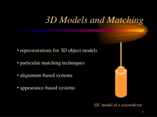
3D Models and Matching • representations for 3D object models • particular matching techniques • alignment-based systems • appearance-based systems GC model of a screwdriver
3D Models • Many different representations have been used to model • 3D objects. • Some are very coarse, just picking up the important features. • Others are very fine, describing the entire surface of the object. • Usually, the recognition procedure depends very much on • the type of model.
Mesh Models Mesh models were originally for computer graphics. With the current availability of range data, they are now used for 3D object recognition. What types of features can we extract from meshes for matching ? In addition to matching, they can be used for verification.
Surface-Edge-Vertex Models SEV models are at the opposite extreme from mesh models. They specify the (usually linear) features that would be extracted from 2D or 3D data. They are suitable for objects with sharp edges and corners that are easily detectable and characterize the object. surface edge vertex surface surface
Generalized-Cylinders A generalized cylinder is a volumetric primitive defined by: • a space curve axis • a cross section function This cylinder has - curved axis - varying cross section standard cylinder rectangular cross sections
Generalized-Cylinder Models Generalized cylinder models include: • a set of generalized cylinders • the spatial relationships among them • the global properties of the object 2 1 2 3 1 How can we describe the attributes of the cylinders and of their connections? 3
Finding GCs in Intensity Data Generalized cylinder models have been used for several different classes of objects: - airplanes (Brooks) - animals (Marr and Nishihara) - humans (Medioni) - human anatomy (Zhenrong Qian) The 2D projections of standard GCs are - ribbons - ellipses
Octrees - Octrees are 8-ary tree structures that compress a voxel representation of a 3D object. - Kari Puli used them to represent the 3D objects during the space carving process. - They are sometimes used for medical object representation. M 5 1 0 4 0 4 6 2 F F F E F F F E 0 1 2 3 4 5 6 7
Superquadrics • Superquadrics are parameterized equations that • describe solid shapes algebraically. • They have been used for graphics and for representing • some organs of the human body, ie. the heart.
2D Deformable Models A 2D deformable model or snake is a function that is fit to some real data, along its contours. The fitting mimizes: - internal energy of the contour (smoothness) - image energy (fit to data) - external energy (user- defined constraints)
3D Deformable Models In 3D, the snake concept becomes a balloon that expands to fill a point cloud of 3D data.
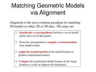
Matching Geometric Modelsvia Alignment Alignment is the most common paradigm for matching 3D models to either 2D or 3D data. The steps are: 1. hypothesize a correspondence between a set of model points and a set of data points 2. From the correspondence compute a transformation from model to data 3. Apply the transformation to the model features to produce transformed features 4. Compare the transformed model features to the image features to verify or disprove the hypothesis
2D-3D Alignment • single 2D images of the objects • 3D object models • - full 3D models, such as GC or SEV • - view class models representing characteristic • views of the objects
View Classes and Viewing Sphere • The space of view points can be • partitioned into a finite set of • characteristic views. • Each view class represents a set of • view points that have something • in common, such as: • 1. same surfaces are visible • 2. same line segments are visible • 3. relational distance between pairs of them is small V v
3 View Classes of a Cube 1 surface 2 surfaces 3 surfaces
TRIBORS: view class matching of polyhedral objects • Each object had 4-5 view classes (hand selected) • The representation of a view class for matching included: • - triplets of line segments visible in that class • - the probability of detectability of each triplet determined • by graphics simulation
RIO: Relational Indexing for Object Recognition • RIO worked with more complex parts that could have • - planar surfaces • - cylindrical surfaces • - threads
Object Representation in RIO • 3D objects are represented by a 3D mesh and set of 2D view classes. • Each view class is represented by an attributed graph whose • nodes are features and whose attributed edges are relationships. • For purposes of indexing, attributed graphs are stored as • sets of 2-graphs, graphs with 2 nodes and 2 relationships. share an arc coaxial arc cluster ellipse
RIO Features ellipses coaxials coaxials-multi parallel lines junctions triples close and far L V Y Z U
RIO Relationships • share one arc • share one line • share two lines • coaxial • close at extremal points • bounding box encloses / enclosed by
Hexnut Object What other features and relationships can you find?
Graph and 2-Graph Representations 1 coaxials- multi encloses 1 1 2 3 2 3 3 2 encloses 2 ellipse e e e c encloses 3 parallel lines coaxial
Relational Indexing for Recognition Preprocessing (off-line) Phase • for each model view Mi in the database • encode each 2-graph of Mi to produce an index • store Mi and associated information in the indexed • bin of a hash table H
Matching (on-line) phase • Construct a relational (2-graph) description D for the scene • For each 2-graph G of D • Select the Mis with high votes as possible hypotheses • Verify or disprove via alignment, using the 3D meshes • encode it, producing an index to access the hash table H • cast a vote for each Mi in the associated bin
RIO Verifications incorrect hypothesis 1. The matched features of the hypothesized object are used to determine its pose. 2. The 3D mesh of the object is used to project all its features onto the image. 3. A verification procedure checks how well the object features line up with edges on the image.
Functional Models(Stark and Bowyer) • Classes of objects are defined through their functions. • Knowledge primitives are parameterized procedures • that check for basic physical concepts such as • - dimensions • - orientation • - proximity • - stability • - clearance • - enclosure
Functional Recognition Procedure • Segment the range data into surfaces • Use a bottom-up analysis to determine all functional properties • From this, construct indexes that are used to rank order the • possible objects and prune away the impossible ones • Use a top-down approach to fully test for the most highly • ranked categories. What are the strengths and weaknesses of this approach?
3D-3D Alignment of Mesh Models to Mesh Data • Older Work: match 3D features such as 3D edges and junctions • or surface patches • More Recent Work: match surface signatures - curvature at a point - curvature histogram in the neighborhood of a point - Medioni’s splashes - Johnson and Hebert’s spin images *
The Spin Image Signature P is the selected vertex. X is a contributing point of the mesh. is the perpendicular distance from X to P’s surface normal. is the signed perpendicular distance from X to P’s tangent plane. X n tangent plane at P P
Spin Image Construction • A spin image is constructed • - about a specified oriented point o of the object surface • - with respect to a set of contributing points C, which is • controlled by maximum distance and angle from o. • It is stored as an array of accumulators S(,) computed via: • For each point c in C(o) • 1. compute and for c. • 2. increment S (,) o
Spin Image Matching ala Sal Ruiz
Spin Images Object Recognition Offline: Compute spin images of each vertex of the object model(s) 1. Compute spin images at selected points of a scene. 2. Compare scene spin images with model scene images by correlation or related method. 3. Group strong matches as in pose clustering and eliminate outliers. 4. Use the winning pose transformation to align the model to the image points and verify or disprove.