Algorithm Analysis
Learn about estimating and reducing algorithm time, using mathematical analysis, execution time of algorithms, and growth rates. Explore common growth rates and big O notation.

Algorithm Analysis
E N D
Presentation Transcript
Algorithm Analysis CENG 707
Algorithmic Performance There are two aspects of algorithmic performance: • Time • Instructions take time. • How fast does the algorithm perform? • What affects its runtime? • Space • Data structures take space • What kind of data structures can be used? • How does choice of data structure affect the runtime? • We will focus on time: • How to estimate the time required for an algorithm • How to reduce the time required CENG 707
Analysis of Algorithms • When we analyze algorithms, we should employ mathematical techniques that analyze algorithms independently of specific implementations, computers, or data. • To analyze algorithms: • First, we start to count the number of significant operations in a particular solution to assess its efficiency. • Then, we will express the efficiency of algorithms using growth functions. CENG 707
The Execution Time of Algorithms • Each operation in an algorithm (or a program) has a cost. Each operation takes a certain CPU time. count = count + 1; take a certain amount of time, but it is constant A sequence of operations: count = count + 1; Cost: c1 sum = sum + count; Cost: c2 Total Cost = c1 + c2 CENG 707
The Execution Time of Algorithms (cont.) Example: Simple If-Statement CostTimes if (n < 0) c1 1 absval = -n c2 1 else absval = n; c3 1 Total Cost <= c1 + max(c2,c3) CENG 707
The Execution Time of Algorithms (cont.) Example: Simple Loop CostTimes i = 1; c1 1 sum = 0; c2 1 while (i <= n) { c3 n+1 i = i + 1; c4 n sum = sum + i; c5 n } Total Cost = c1 + c2 + (n+1)*c3 + n*c4 + n*c5 The time required for this algorithm is proportional to n CENG 707
The Execution Time of Algorithms (cont.) Example: Nested Loop CostTimes i=1; c1 1 sum = 0; c2 1 while (i <= n) { c3 n+1 j=1; c4 n while (j <= n) { c5 n*(n+1) sum = sum + i; c6 n*n j = j + 1; c7 n*n } i = i +1; c8 n } Total Cost = c1 + c2 + (n+1)*c3 + n*c4 + n*(n+1)*c5+n*n*c6+n*n*c7+n*c8 The time required for this algorithm is proportional to n2 CENG 707
General Rules for Estimation • Loops: The running time of a loop is at most the running time of the statements inside of that loop times the number of iterations. • Nested Loops: Running time of a nested loop containing a statement in the inner most loop is the running time of statement multiplied by the product of the sized of all loops. • Consecutive Statements: Just add the running times of those consecutive statements. • If/Else: Never more than the running time of the test plus the larger of running times of S1 and S2. CENG 707
Algorithm Growth Rates • We measure an algorithm’s time requirement as a function of the problem size. • Problem size depends on the application: e.g. number of elements in a list for a sorting algorithm, the number disks for towers of hanoi. • So, for instance, we say that (if the problem size is n) • Algorithm A requires 5*n2 time units to solve a problem of size n. • Algorithm B requires 7*n time units to solve a problem of size n. • The most important thing to learn is how quickly the algorithm’s time requirement grows as a function of the problem size. • Algorithm A requires time proportional to n2. • Algorithm B requires time proportional to n. • An algorithm’s proportional time requirement is known as growth rate. • We can compare the efficiency of two algorithms by comparing their growth rates. CENG 707
Algorithm Growth Rates (cont.) Time requirements as a function of the problem size n CENG 707
Common Growth Rates CENG 707
Figure 6.1 Running times for small inputs CENG 707
Figure 6.2 Running times for moderate inputs CENG 707
Order-of-Magnitude Analysis and Big 0 Notation • If Algorithm A requires time proportional to f(n), Algorithm A is said to be order f(n), and it is denoted as O(f(n)). • The function f(n) is called the algorithm’s growth-rate function. • Since the capital O is used in the notation, this notation is called the Big O notation. • If Algorithm A requires time proportional to n2, it is O(n2). • If Algorithm A requires time proportional to n, it is O(n). CENG 707
Definition of the Order of an Algorithm Definition: Algorithm A is order f(n) – denoted as O(f(n)) – if constants k and n0 exist such that A requires no more than k*f(n) time units to solve a problem of size n n0. • The requirement of n n0 in the definition of O(f(n)) formalizes the notion of sufficiently large problems. • In general, many values of k and n0 can satisfy this definition. CENG 707
Order of an Algorithm • Suppose an algorithm requires n2–3*n+10 seconds to solve a problem size n. If constants k and n0 exist such that k*n2 > n2–3*n+10 for all n n0 . the algorithm is order n2(In fact, k is 3 and n0 is 2) 3*n2 > n2–3*n+10 for all n 2 . Thus, the algorithm requires no more than k*n2 time units for n n0 , So it is O(n2) CENG 707
Growth-Rate Functions O(1) Time requirement is constant, and it is independent of the problem’s size. O(log2n) Time requirement for a logarithmic algorithm increases increases slowly as the problem size increases. O(n) Time requirement for a linear algorithm increases directly with the size of the problem. O(n*log2n) Time requirement for a n*log2n algorithm increases more rapidly than a linear algorithm. O(n2) Time requirement for a quadratic algorithm increases rapidly with the size of the problem. O(n3) Time requirement for a cubic algorithm increases more rapidly with the size of the problem than the time requirement for a quadratic algorithm. O(2n) As the size of the problem increases, the time requirement for an exponential algorithm increases too rapidly to be practical. CENG 707
Growth-Rate Functions • If an algorithm takes 1 second to run with the problem size 8, what is the time requirement (approximately) for that algorithm with the problem size 16? • If its order is: O(1) T(n) = 1 second O(log2n) T(n) = (1*log216) / log28 = 4/3 seconds O(n) T(n) = (1*16) / 8 = 2 seconds O(n*log2n) T(n) = (1*16*log216) / 8*log28 = 8/3 seconds O(n2) T(n) = (1*162) / 82 = 4 seconds O(n3) T(n) = (1*163) / 83 = 8 seconds O(2n) T(n) = (1*216) / 28 = 28 seconds = 256 seconds CENG 707
Properties of Growth-Rate Functions • We can ignore low-order terms in an algorithm’s growth-rate function. • If an algorithm is O(n3+4n2+3n), it is also O(n3). • We only use the higher-order term as algorithm’s growth-rate function. • We can ignore a multiplicative constant in the higher-order term of an algorithm’s growth-rate function. • If an algorithm is O(5n3), it is also O(n3). • O(f(n)) + O(g(n)) = O(f(n)+g(n)) • We can combine growth-rate functions. • If an algorithm is O(n3) + O(4n), it is also O(n3 +4n2) So, it is O(n3). • Similar rules hold for multiplication. CENG 707
Some Mathematical Facts • Some mathematical equalities are: CENG 707
Growth-Rate Functions – Example1 CostTimes i = 1; c1 1 sum = 0; c2 1 while (i <= n) { c3 n+1 i = i + 1; c4 n sum = sum + i; c5 n } T(n) = c1 + c2 + (n+1)*c3 + n*c4 + n*c5 = (c3+c4+c5)*n + (c1+c2+c3) = a*n + b So, the growth-rate function for this algorithm is O(n) CENG 707
Growth-Rate Functions – Example2 CostTimes i=1; c1 1 sum = 0; c2 1 while (i <= n) { c3 n+1 j=1; c4 n while (j <= n) { c5 n*(n+1) sum = sum + i; c6 n*n j = j + 1; c7 n*n } i = i +1; c8 n } T(n) = c1 + c2 + (n+1)*c3 + n*c4 + n*(n+1)*c5+n*n*c6+n*n*c7+n*c8 = (c5+c6+c7)*n2 + (c3+c4+c5+c8)*n + (c1+c2+c3) = a*n2 + b*n + c So, the growth-rate function for this algorithm is O(n2) CENG 707
Growth-Rate Functions – Example3 CostTimes for (i=1; i<=n; i++) c1 n+1 for (j=1; j<=i; j++) c2 for (k=1; k<=j; k++) c3 x=x+1; c4 T(n) = c1*(n+1) + c2*( ) + c3* ( ) + c4*( ) = a*n3 + b*n2 + c*n + d So, the growth-rate function for this algorithm is O(n3) CENG 707
What to Analyze • An algorithm can require different times to solve different problems of the same size. • Eg. Searching an item in a list of n elements using sequential search. Cost: 1,2,...,n • Worst-Case Analysis –The maximum amount of time that an algorithm require to solve a problem of size n. • This gives an upper bound for the time complexity of an algorithm. • Normally, we try to find worst-case behavior of an algorithm. • Best-Case Analysis –The minimum amount of time that an algorithm require to solve a problem of size n. • The best case behavior of an algorithm is NOT so useful. • Average-Case Analysis –The average amount of time that an algorithm require to solve a problem of size n. • Sometimes, it is difficult to find the average-case behavior of an algorithm. • We have to look at all possible data organizations of a given size n, and their distribution probabilities of these organizations. • Worst-case analysis is more common than average-case analysis. CENG 707
What is Important? • We have to weigh the trade-offs between an algorithm’s time requirement and its memory requirements. • We have to compare algorithms for both style and efficiency. • The analysis should focus on gross differences in efficiency and not reward coding tricks that save small amount of time. • That is, there is no need for coding tricks if the gain is not too much. • Easily understandable program is also important. • Order-of-magnitude analysis focuses on large problems. CENG 707
Sequential Search int sequentialSearch(int a[], int x, int n) { int i; for (i = 0; i < n && a[i]!= x; i++); if (i == n) return –1; return i; } Unsuccessful Search: O(n) Successful Search: Best-Case:item is in the first location of the array O(1) Worst-Case:item is in the last location of the array O(n) Average-Case: The number of key comparisons 1, 2, ..., n O(n) CENG 707
Binary Search • Array must be sorted. • at each step we reduce the length of the array to be searched by half. • (e.g. array size = 1 million => 20 comparisons needed to locate any item) low mid high CENG 707
Binary Search Algorithm int binarySearch(int a[], int size, int x) { int low =0; int high = size – 1; int mid; // mid will be the index of //target when it’s found. while (low <= high) { mid = (low + high)/2; if (a[mid] < x) low = mid + 1; else if (a[mid] > x) high = mid – 1; else return mid; } return –1; } CENG 707
Binary Search – Analysis • For an unsuccessful search: • The number of iterations in the loop is log2n + 1 O(log2n) • For a successful search: • Best-Case: The number of iterations is 1. O(1) • Worst-Case:The number of iterations is log2n +1 O(log2n) • Average-Case: The avg. # of iterations < log2n O(log2n) 0 1 2 3 4 5 6 7 an array with size 8 3 2 3 1 3 2 3 4 # of iterations The average # of iterations = 21/8 < log28 CENG 707
How much better is O(log2n)? nO(log2n) 16 4 64 6 256 8 1024 (1KB) 10 16,384 14 131,072 17 262,144 18 524,288 19 1,048,576 (1MB) 20 1,073,741,824 (1GB) 30 CENG 707