Fluid Mechanics
Fluid Mechanics. Topics Covered. Fluid statics Pressure measurement Fluids in motion Pump performance parameters. Fluid Statics. Fluid statics : study of fluids at rest

Fluid Mechanics
E N D
Presentation Transcript
Topics Covered • Fluid statics • Pressure measurement • Fluids in motion • Pump performance parameters
Fluid Statics • Fluid statics: study of fluids at rest • Different from fluid dynamics in that it concerns pressure forces perpendicular to a plane (referred to as hydrostatic pressure) • If you pick any one point in a static fluid, that point is going to have a specific pressure intensity associated with it: • P = F/A where • P = pressure in Pascals (Pa, lb/ft2) or Newtons (N, kg/m2) • F = normal forces acting on an area (lbs or kgs) • A = area over which the force is acting (ft2 or m2)
Fluid Statics • This equation, P = F/A, can be used to calculate pressure on the bottom of a tank filled with a liquid (or.. at any depth) F = V = fluid specific wt (N/m3), V = volume (m3) h P = h h = depth of water (m or ft) P1
Fluid Statics • Pressure is the same at all points at equal height from the bottom of the tank • Point: temp doesn’t make that much difference in pressure for most aquaculture situations • Example: What is the pressure at a point 12 ft. from the bottom of a tank containing freshwater at 80oF vs. 40oF? • 80oF = 62.22 lb/ft3; thus, P = (62.22)(12) = 746.4 lb/ft 2 • 40oF = 62.43 lb/ft3; thus, P = (62.43)(12) = 749.2 lb/ft2
Fluids in Motion • Fundamental equation: Qin – Qout = storage • Qin = quantity flowing into the system; Qout = that flowing out; the difference is what’s stored • If we divide storage by a time interval (e.g., seconds), we can determine rate of filling or draining • Very applicable to tanks, ponds, etc. • Problem: A 100,000 m3 pond (about 10 ha) is continuously filled with water from a distribution canal at 100 m3 per minute. Assuming that the pond was initially full, but some idiot removed too many flashboards in the exit gate and it was draining at 200 m3 per minute, how long will it take to be essentially empty? • Volume/flow rate = 100,000 m3/200 m3/min = 500 min
Closed System Fluids in Motion • Let’s say we’re not dealing with a system open to the atmosphere (e.g., a pipe vs. a pond) • There’s no storage potential, so Q1 = Q2, a mass balance equation • For essentially incompressible fluids such as water, the equation becomes V1A1 = V2A2,; where V = velocity (m/s) and A = area (m2) • Can be used to estimate flow velocity along a pipe, especially where constrictions are concerned • Example: If one end of a pipe has a diameter of 0.1 m and a flow rate of 0.05 m/s, what will be the flow velocity at a constriction in the other end having a diameter of 0.01 m? Ans. V2 = 0.5 m/s
Bernoulli’s Equation • Z1 + (P1/) + (V12/2g) = Z2 + (P2/) + (V22/2g) • Wow! Z = pressure head, V2/2g = velocity head (heard of these?), 2g = (2)(32.2) for Eng. System • If we’re trying to figure out how quickly a tank will drain, we use this equation in a simplified form: Z = V2/2g • Example: If the vertical distance between the top of the water in a tank and the centerline of it’s discharge pipe is 14 ft, what is the initial discharge velocity of the water leaving the tank? Ans. = 30 ft/s • Can you think of any applications for this?
Reality • In actuality, fluids have losses due to friction in the pipes and minor losses associated with tees, elbows, valves, etc. • Also, there is usually an external power source (pump). The equation becomes Z1 + (P1/) + (V12/2g) + EP = Z2 + (P2/) + (V22/2g) + hm + hf • If no pump (gravity flow), EP = 0. EP is energy from the pump, hm and hf = minor and frictional head losses, resp.
Minor Losses • These are losses in pressure associated with the fluid encountering: • restrictions in the system (valves) • changes in direction (elbows, bends, tees, etc.) • changes in pipe size (reducers, expanders) • losses associated with fluid entering or leaving a pipe • Screens, foot valves also create minor losses • A loss coefficient, K, is associated with each component • total minor losses, hm, = K(V2/2g)
Your Inevitable Example • Calculate the total minor losses associated with the pipe to the right when the gate valve is ¾ open, D = 6 in., d = 3 in. and V = 2ft/s • Refer to the previous table • Ans: hm = 0.15 ft • hm = (0.9+1.15+0.4)(2)2 (2)(32.2)
Pipe Friction Losses • Caused by friction generated by the movement of the fluid against the walls of pipes, fittings, etc. • Magnitude of the loss depends upon: • Internal pipe diameter • Fluid velocity • Roughness of internal pipe surfaces • Physical properties of the fluid (e.g., density, viscocity) f = function ( ) VD , D Where, f = friction factor; D = inside pipe diameter; V = fluid viscocity; = absolute roughness; = fluid density; and = absolute viscocity
Pipe Friction Losses • Simplified, f = 64/RN Is known as the Reynold’s number, RN, also written as VD/v VD , /D /D Is called the relative roughness and is the ratio of the absolute roughness to inside pipe diameter
Darcy-Weisbach Equation • hf = f(L/D)(V2/2g) • Where hf = pipe friction head loss (m/ft); f = friction factor; L = total straight length of pipe (m/ft); D = inside pipe diameter (m/ft); V = fluid velocity (m/s or ft/s); g = gravitational constant (m/s2 or ft/s2) • Problem: Water at 20 C is flowing through a 500 m section of 10 cm diameter old cast iron pipe at a velocity of 1.5m/s. Calculate the total friction losses , hf, using the Darcy-Weisbach Equation • Ans.
Answer to Previous • RN = VD/; where or kinematic viscocity is 1 x 10⁻⁶ (trust me on this) • RN = (1.5)(0.1)/.000001 = 150,000 • = .026 (in cm) for cast iron pipe; /D = .00026 m/.1 = .0026 • f = 0.027 where on Moody’s Diagram /D aligns with a Reynold’s Number of 150,000 • hf = (.0027)(500)(1.5)2 = 15.5 m (0.1)(2)(9.81)
Reality • This value, hf is added to hm to arrive at your total losses • Alternative method for frictional losses: Hazen-Williams equation • hf = (10.7LQ1.852)/(C1.852)(D4.87) metric systems • hf = (4.7LQ1.852)/((C1.852)(D4.87) English systems • Where hf = pipe friction losses (m, ft); L = length of piping (m, ft); Q = flow rate (m3/s, ft3/s); C = Hazen-Williams coefficient; and D = pipe diameter (m, ft)
Example • Estimate the friction losses in a 6-in. diameter piping system containing 200 ft of straight pipe, a half-closed gate valve, two close return bends and four ell90s. The water velocity in the pipe is 2.5 ft/s? • hf = (10.7)(145m)(0.014)1.852 (120)1.852(0.152)4.87 = 2.6 ft
OK, what about PUMPING? • Pump’s performance is described by the following parameters: • Capacity • Head • Power • Efficiency • Net positive suction head • Specific speed • Capacity, Q, is the volume of water delivered per unit time by the pump (usually gpm)
Pump Performance • Head is the net work done on a unit of water by the pump and is given by the following equation • Hs = SL + DL + DD + hm + hf + ho + hv • Hs = system head, SL = suction-side lift, DD = water source drawdown, hm = minor losses (as previous), hf = friction losses (as previous), ho = operating head pressure, and hv = velocity head (V2/2g) • Suction and discharge static lifts are measured when the system is not operating • DD, drawdown, is decline of the water surface elevation of the source water due to pumping (mainly for wells) • DD, hm, hf, ho and hv all increase with increased pumping capacity, Q
Pump Performance: power • Power to operate a pump is directly proportional to discharge head, specific gravity of the fluid (water), and is inversely proportional to pump efficiency • Power imparted to the water by the pump is referred to as water horsepower • WHP = QHS/K; where Q = pump capacity or discharge, H = head, S = specific gravity, K = 3,960 for WHP in hp and Q in gpm. • WHP can also equal Q(TDH)/3,960 where TDH = total dynamic head (sum of all losses while pump is operating)
Pump Performance: efficiency • Usually determined by brake horsepower (BHP) • BHP = power that must be applied to the shaft of the pump by a motor to turn the impeller and impart power to the water • Ep= 100(WHP/BHP) = output/input • Epnever equals 100% due to energy losses such as friction in bearings around shaft, moving water against pump housing, etc. • Centrifugal pump efficiencies range from 25-85% • If pump is incorrectly sized, Ep is lower.
Pump Performance: suction head • Conditions on the suction side of a pump can impart limitations on pumping systems • What is the elevation of the pump relative to the water source? • Static suction lift (SL) = vertical distance from water surface to centerline of the pump • SL is positive if pump is above water surface, negative if below • Total suction head (Hs) = SL + friction losses + velocity head: Hs = SL + (hm + hf) + V2s/2g
Pump Performance Curves • Report data on a pump relevant to head, efficiency, power requirements, and net positive suction head to capacity • Each pump is unique dependent upon its geometry and dimensions of the impeller and casing • Reported as an average or as the poorest performance
Characteristic Pump Curves • Head as capacity • Efficiency as capacity , up to a point • BHP as capacity , also up to a point • REM: • BHP = 100QHS/Ep3,960