Download
1 / 39
390 likes | 580 Vues
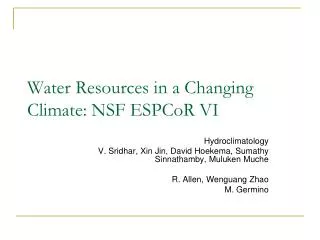
Water Resources in a Changing Climate: NSF ESPCoR VI. Hydroclimatology V. Sridhar, Xin Jin, David Hoekema, Sumathy Sinnathamby, Muluken Muche R. Allen, Wenguang Zhao M. Germino. Background and Context. Region-wide warming Precipitation change Decline of snowpack

E N D
Water Resources in a Changing Climate: NSF ESPCoR VI Hydroclimatology V. Sridhar, Xin Jin, David Hoekema, Sumathy Sinnathamby, Muluken Muche R. Allen, Wenguang Zhao M. Germino
Background and Context • Region-wide warming • Precipitation change • Decline of snowpack • Earlier spring runoff and • Decline in summer streamflow trends
Research Questions • How will future climate change impact water resources? • Hydro - Climate • Hydro - Economic / Policy • Hydro - Ecology
Research Questions • Hydro-climate interactions • What are the relationships between climate change, vegetation, snow pack, and the resulting stream flows in managed and unmanaged river systems? • How will aquifer systems exchange with surface and groundwater under various climate change scenarios? • What will both the supply and demand on water be in these systems under various climate change scenarios?
How will fire and invasive species (cheat grass, some bunchgrasses) impact: Rates and durations of ET fluxes from desert systems? Changes in infiltration patterns for precipitation? Interactions of ET, infiltration, thermal profiles and microbial populations and feedbacks? Erosion and Sedimentation in Tributaries of the Snake and Salmon basins? Hydroclimate Bio Interactions
Focus Area 2009-2011 • Research 1: Advance our ability to model surface energy balance processes • Tasks: Use of scintillometer and eddy covariance (EC) systems to measure sensible (H) and latent (LE) heat fluxes in desert and timber • Research 2:Advancement in Basin scale Hydrologic Forecasting – verification and operation under climate change scenarios • Task1 : Operate, test and calibrate the CIG Variable Infiltration Capacity (VIC) model and combine with the groundwater model • Task2: Implement VIC –groundwater model and evaluate the reservoir optimization techniques
Scintillometry • Use to Retrieve Sensible Heat Flux (H) over large, integrated transects • Use to improve components in METRIC and VIC • Reduce variances • Use to derive ET experimentally • Determine how soil water meters out from desert and lodgepole
Scintillometers to measure surface heat flux densities Transmitter Receiver Surface Energy Balance Processes----Large aperture scintillometer--transmitter (left) and 3 intercompared receivers (right) purchased by Idaho EPSCoR RII
Scintillometer – Idaho RII Deployments • Three systems (BSU, ISU, UI) • Three deployments • Sage brush -- Snake River Plain • Cheat grass or recent burn – Snake River Plain • Timber – Upper Reaches
Idaho RII: Sagebrush Deployment Sage brush ecosystem located west of Hollister, Idaho.
LodgePole Pine Site --- Macks Inn Area
Scintillometers measure only Sensible Heat flux (H)ET is calculated as a residual of the energy balance ET = Rn – G – H Net radiation, Rn, and soil heat flux, G, must be measured All error in Rn, G and H transfer into ET
Choose parameters to be calibrated. In this study, 7 parameters were chosen recommendation Divide the range of each parameter into equal space Run VIC and routing with one parameter changed and the others unchanged. Obtaining new RMSE. Choose observation locations to be used as reference. In this study, 6 locations were chosen Calculate sensitivity for each observation yi (i=1,…,n) over each parameter bj (j=1,…,p). Divide the Snake River Basin into 6 sub-basins and select the new set of parameters that make the RMSE minimum and apply it to the VIC Construct nxp Jacobian matrix and calculate CSSj Identify the most sensitive parameters (with the biggest CSSj) end Preliminary VIC model calibration & Flowchart for sensitivity analysis • Ws fraction of maximum soil moisture where non-linear baseflow occurs
VIC model calibration results (all 6 locations, 1928 - 1978) VIC model validation results (all 6 locations, 1979 - 2005)
VIC model calibration results (at Heise) Default calibrated from University of Washington calibrated
Parameter Selection for the SWAT Model Snowmelt and snow formation parameter Ground water parameter Soil parameter Surface Runoff parameter
Snake River watershed Salmon River watershed Decreasing trend in monthly discharges
White bird Yellowpine Krassel Ranger A1b A1b A1b Average annual flow (cms) A2 A2 A2 B1 B1 B1 ECHAM GISS IPSL
Milner Oxbow A1b A1b ECHAM Average annual flow (cms) GISS IPSL A2 A2 B1 B1
Milner Oxbow A1b A1b Snake River watershed Mean Monthly flow (cms) A2 A2 B1 B1
Flow Distribution & Points of Interest (POI) Points of interest were chosen from which projected flows could be distributed to simulate upstream reach gain contributions. As represented in the chart below, we selected six points of interest that cover 90% of the flow in the upper SRB. • Six Points of Interest • Heise (Snake River) • Rexburg (Henry’s Fork) • Milner (Snake River) • Parma (Boise River) • Payette (Payette River) • Oxbow (Snake River) • 58% • +32% • 90 % Total
Reach Gain Simulation Calculations • Monthly Natural flow (sum of upstream reaches) • Where, • NFm = monthly natural flow at reach d • d = downstream reach (or point of interest) • u = furthest upstream reach • xi = any given reach between u and d • Annual Natural Flow (sum of monthly Natural Flows) • Where, NFm,1 = natural monthly flow in October, NFM,2 = natural monthly flow in November…. The first step of the reach gain simulation method is to categorize flow based on a range of historic annual natural flows. The equations for calculating natural flow from IDWR historic reach gains are presented here.
Flow Categorization Henry’s Fork Flow categorization is based on annual flows while simulation of these flows are based on monthly distributions of the projected flow. Along the Henry’s Fork flows are categorized with a range of 300,000 acre-feet per category. Flow Range per Category: 3000 (100 acre-feet) Minimum: 13678 Maximum: 40697 Mean: 24768
Irrigation Shortage Comparison: Historic vs. Simulated (1980-2005) A comparison between SRPM calculated irrigation shortages as represented by historic and simulated reach gains reveals that the reach gain simulation method was able to provide perfect replication of historic irrigation shortages in the river between the years 1980 and 2005.
Payette Watershed-Future Climate: Echam-5 Deadwood Dam Cascade Dam Black Canyon Dam
Run VIC model to generate the infiltration, evapotransporation (ET), runoff and baseflow at each cell of unsaturated zone Infiltration, ET Water content Run MODFLOW and generate recharge, water content Add a fraction of recharge from MODFLOW the baseflow in VIC output Run VIC routing model No Reaching time step limit Yes Stop VIC+MODFLOW flowchart