Comparing Means from Two Samples
Statistics 111 – Lecture 14. Comparing Means from Two Samples. and. One-Sample Inference for Proportions. Administrative Notes. Homework 5 is posted on website Due Wednesday, July 1 st. Outline. Two Sample Z-test (known variance) Two Sample t -test (unknown variance)

Comparing Means from Two Samples
E N D
Presentation Transcript
Statistics 111 – Lecture 14 Comparing Meansfrom Two Samples and One-Sample Inference for Proportions Stat 111 - Lecture 14 - Two Means
Administrative Notes • Homework 5 is posted on website • Due Wednesday, July 1st Stat 111 - Lecture 14 - Two Means
Outline • Two Sample Z-test (known variance) • Two Sample t-test (unknown variance) • Matched Pair Test and Examples • Tests and Intervals for Proportions (Chapter 8) Stat 111 - Lecture 14 - Two Means
Comparing Two Samples • Up to now, we have looked at inference for one sample of continuous data • Our next focus in this course is comparing the data from two different samples • For now, we will assume that these two different samples are independent of each other and come from two distinct populations Population 1:1 , 1 Population 2: 2 , 2 Sample 1: , s1 Sample 2: , s2 Stat 111 - Lecture 14 - Means
Blackout Baby Boom Revisited • Nine months (Monday, August 8th) after Nov 1965 blackout, NY Times claimed an increased birth rate • Already looked at single two-week sample: found no significant difference from usual rate (430 births/day) • What if we instead look at difference between weekends and weekdays? Weekdays Weekends Stat 111 - Lecture 14 - Means
Two-Sample Z test • We want to test the null hypothesis that the two populations have different means • H0: 1 = 2 or equivalently, 1 - 2 = 0 • Two-sided alternative hypothesis: 1 - 2 0 • If we assume our population SDs 1 and 2 are known, we can calculate a two-sample Z statistic: • We can then calculate a p-value from this Z statistic using the standard normal distribution Stat 111 - Lecture 14 - Means
Two-Sample Z test for Blackout Data • To use Z test, we need to assume that our pop. SDs are known: 1 = s1 = 21.7 and 2 = s2 = 24.5 • From normal table, P(Z > 7.5) is less than 0.0002, so our p-value = 2 P(Z > 7.5) is less than 0.0004 • Conclusion here is a significant difference between birth rates on weekends and weekdays • We don’t usually know the population SDs, so we need a method for unknown 1 and 2 Stat 111 - Lecture 14 - Two Means
Two-Sample t test • We still want to test the null hypothesis that the two populations have equal means (H0: 1 - 2 = 0) • If 1 and 2 are unknown, then we need to use the sample SDs s1 and s2 instead, which gives us the two-sample T statistic: • The p-value is calculated using the t distribution, but what degrees of freedom do we use? • df can be complicated and often is calculated by software • Simpler and more conservative: set degrees of freedom equal to the smaller of (n1-1) or (n2-1) Stat 111 - Lecture 14 - Two Means
Two-Sample t test for Blackout Data • To use t test, we need to use our sample standard deviations s1 = 21.7 and s2 = 24.5 • We need to look up the tail probabilities using the t distribution • Degrees of freedom is the smaller of n1-1 = 22 or n2-1 = 7 Stat 111 - Lecture 14 - Two Means
Two-Sample t test for Blackout Data • From t-table with df = 7, we see that P(T > 7.5) < 0.0005 • If our alternative hypothesis is two-sided, then we know that our p-value < 2 0.0005 = 0.001 • We reject the null hypothesis at -level of 0.05 and conclude there is a significant difference between birth rates on weekends and weekdays • Same result as Z-test, but we are a little more conservative Stat 111 - Lecture 14 - Two Means
Two-Sample Confidence Intervals • In addition to two sample t-tests, we can also use the t distribution to construct confidence intervals for the mean difference • When 1 and 2 are unknown, we can form the following 100·C% confidence interval for the mean difference 1 - 2 : • The critical value tk* is calculated from a t distribution with degrees of freedom k • k is equal to the smaller of (n1-1) and (n2-1) Stat 111 - Lecture 14 - Two Means
Confidence Interval for Blackout Data • We can calculate a 95% confidence interval for the mean difference between birth rates on weekdays and weekends: • We get our critical value tk* = 2.365 is calculated from a t distribution with 7 degrees of freedom, so our 95% confidence interval is: • Since zero is not contained in this interval, we know the difference is statistically significant! Stat 111 - Lecture 14 - Two Means
Matched Pairs • Sometimes the two samples that are being compared are matched pairs (not independent) • Example: Sentences for crack versus powder cocaine • We could test for the mean difference between X1 = crack sentences and X2 = powder sentences • However, we realize that these data are paired: each row of sentences have a matching quantity of cocaine • Our t-test for two independent samples ignores this relationship Stat 111 - Lecture 14 - Two Means
Matched Pairs Test • First, calculate the difference d = X1 - X2 for each pair • Then, calculate the mean and SD of the differences d Stat 111 - Lecture 14 - Two Means
Matched Pairs Test • Instead of a two-sample test for the difference between X1 and X2, we do a one-sample test on the difference d • Null hypothesis: mean difference between the two samples is equal to zero H0 : d= 0 versus Ha : d 0 • Usual test statistic when population SD is unknown: • p-value calculated from t-distribution with df = 8 • P(T > 5.24) < 0.0005 so p-value < 0.001 • Difference between crack and powder sentences is statistically significant at -level of 0.05 Stat 111 - Lecture 14 - Two Means
Matched Pairs Confidence Interval • We can also construct a confidence interval for the mean differenced of matched pairs • We can just use the confidence intervals we learned for the one-sample, unknown case • Example: 95% confidence interval for mean difference between crack and powder sentences: Stat 111 - Lecture 14 - Two Means
Summary of Two-Sample Tests • Two independent samples with known 1 and 2 • We use two-sample Z-test with p-values calculated using the standard normal distribution • Two independent samples with unknown 1 and 2 • We use two-sample t-test with p-values calculated using the t distribution with degrees of freedom equal to the smaller of n1-1 and n2-1 • Also can make confidence intervals using t distribution • Two samples that are matched pairs • We first calculate the differences for each pair, and then use our usual one-sample t-test on these differences Stat 111 - Lecture 14 - Two Means
One-Sample Inference for Proportions Stat 111 - Lecture 14 - Two Means
Revisiting Count Data • Chapter 6 and 7 covered inference for the population mean of continuous data • We now return to count data: • Example: Opinion Polls • Xi = 1 if you support Obama, Xi = 0 if not • We call p the population proportion for Xi = 1 • What is the proportion of people who support the war? • What is the proportion of Red Sox fans at Penn? Stat 111 - Lecture 14- One-Sample Proportions
Inference for population proportion p • We will use sample proportion as our best estimate of the unknown population proportion p where Y = sample count • Tool 1: use our sample statistic as the center of an entire confidence interval of likely values for our population parameter Confidence Interval : Estimate ± Margin of Error • Tool 2: Use the data to for a specific hypothesis test • Formulate your null and alternative hypotheses • Calculate the test statistic • Find the p-value for the test statistic Stat 111 - Lecture 14- One-Sample Proportions
Distribution of Sample Proportion • In Chapter 5, we learned that the sample proportion technically has a binomial distribution • However, we also learned that if the sample size is large, the sample proportion approximately follows a Normal distribution with mean and standard deviation: • We will essentially use this approximation throughout chapter 8, so we can make probability calculations using the standard normal table Stat 111 - Lecture 14- One-Sample Proportions
Confidence Interval for a Proportion • We could use our sample proportion as the center of a confidence interval of likely values for the population parameter p: • The width of the interval is a multiple of the standard deviation of the sample proportion • The multiple Z* is calculated from a normal distribution and depends on the confidence level Stat 111 - Lecture 14- One-Sample Proportions
Confidence Interval for a Proportion • One Problem: this margin of error involves the population proportion p, which we don’t actually know! • Solution: substitute in the sample proportion for the population proportion p, which gives us the interval: Stat 111 - Lecture 14- One-Sample Proportions
Example: Red Sox fans at Penn • What proportion of Penn students are Red Sox fans? • Use Stat 111 class survey as sample • Y = 25 out of n = 192 students are Red Sox fans so • 95% confidence interval for the population proportion: • Proportion of Red Sox fans at Penn is probably between 8% and 18% Stat 111 - Lecture 14- One-Sample Proportions
Hypothesis Test for a Proportion • Suppose that we are now interested in using our count data to test a hypothesized population proportion p0 • Example: an older study says that the proportion of Red Sox fans at Penn is 0.10. • Does our sample show a significantly different proportion? • First Step: Null and alternative hypotheses • H0: p = 0.10 vs. Ha: p 0.10 • Second Step: Test Statistic Stat 111 - Lecture 14- One-Sample Proportions
Hypothesis Test for a Proportion • Problem: test statistic involves population proportion p • For confidence intervals, we plugged in sample proportion but for test statistics, we plug in the hypothesized proportion p0 : • Example: test statistic for Red Sox example Stat 111 - Lecture 14- One-Sample Proportions
Hypothesis Test for a Proportion • Third step: need to calculate a p-value for our test statistic using the standard normal distribution • Red Sox Example: Test statistic Z = 1.39 • What is the probability of getting a test statistic as extreme or more extreme than Z = 1.39? ie. P(Z > 1.39) = ? • Two-sided alternative, so p-value = 2P(Z>1.39) = 0.16 • We don’t reject H0 at a =0.05 level, and conclude that Red Sox proportion is not significantly different from p0=0.10 prob = 0.082 Z = 1.39 Stat 111 - Lecture 14- One-Sample Proportions
Another Example • Mass ESP experiment in 1977 Sunday Mirror (UK) • Psychic hired to send readers a mental message about a particular color (out of 5 choices). Readers then mailed back the color that they “received” from psychic • Newspaper declared the experiment a success because, out of 2355 responses, they received 521 correct ones ( ) • Is the proportion of correct answers statistically different than we would expect by chance (p0 = 0.2) ? • H0: p= 0.2 vs. Ha: p 0.2 Stat 111 - Lecture 14- One-Sample Proportions
Mass ESP Example • Calculate a p-value using the standard normal distribution • Two-sided alternative, so p-value = 2P(Z>2.43) = 0.015 • We reject H0 at a =0.05 level, and conclude that the survey proportion is significantly different from p0=0.20 • We could also calculate a 95% confidence interval for p: prob = 0.0075 Z = 2.43 Interval doesn’t contain 0.20 Stat 111 - Lecture 14- One-Sample Proportions
Margin of Error • Confidence intervals for proportion p is centered at the sample proportion and has a margin of error: • Before the study begins, we can calculate the sample size needed for a desired margin of error • Problem: don’t know sample prop. before study begins! • Solution: use which gives us the maximum m • So, if we want a margin of error less than m, we need Stat 111 - Lecture 14- One-Sample Proportions
Margin of Error Examples • Red Sox Example: how many students should I poll in order to have a margin of error less than 5% in a 95% confidence interval? • We would need a sample size of 385 students • ESP example: how many responses must newspaper receive to have a margin of error less than 1% in a 95% confidence interval? Stat 111 - Lecture 14- One-Sample Proportions
Next Class - Lecture 15 • Two-Sample Inference for Proportions • Moore, McCabe and Craig: Section 8.2 Stat 111 - Lecture 14- One-Sample Proportions