
Next week’s assignment:
Next week’s assignment:. 1) Using clumping indexes, LAI and values for a conifer stand (Loblolly pine forest, Duke Univ.) and for a Eucalyptus plantation (New Zealand), calculate their Monthly GPP (potential GPP). - Loblolly pine: = 2.37 gC MJ -1 APAR

Next week’s assignment:
E N D
Presentation Transcript
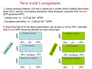
Next week’s assignment: 1) Using clumping indexes, LAI and values for a conifer stand (Loblolly pine forest, Duke Univ.) and for a Eucalyptus plantation (New Zealand), calculate their Monthly GPP(potential GPP). - Loblolly pine: = 2.37 gC MJ-1 APAR - Eucalyptus plantation: = 3.85 gC MJ-1 APAR 2) Assuming that all of the above parameters vary by plus or minus 20%, calculate how Annual GPP would be affected for each forest type. , Clumping =constant , Clumping =constant GPP GPP +20% -20% +20% LAI -20% LAI , LAI =constant , LAI =constant Loblolly pine GPP GPP Eucalyptus +20% -20% +20% Clumping -20% Clumping Clumping, LAI =constant Clumping, LAI =constant GPP GPP +20% -20% +20% -20%
Using clumping indexes, LAI and values for a conifer stand (Loblolly pine forest, Duke Univ.) and for a Eucalyptus plantation (New Zealand), calculate their Monthly GPP(potential GPP). • Loblolly pine: = 2.37 gC MJ-1 APAR ; • - Eucalyptus plantation: = 3.85 gC MJ-1 APAR
2) Assuming that all of the above parameters vary by plus or minus 20%, calculate how Annual GPP would be affected for each forest type. Actual GPPs Pine = 2500 gC m-2 year-1 Euca = 3300 gC m-2 year-1
“Productivity” equation Light supply and light capture GPP = {f(D)f(T)f() f(CO2)}*APAR Constraints to photosynthesis Maximum potential photosynthesis rate Canopy quantum efficiency = Aleaf/ PAR Aleaf= ca (1- ci/ca) * gleaf
At the same time, H2O vapor moves out of the leaf by diffusion (but really H2O vapor moves both directions) CO2 moves from the air to the leaf to the chloroplast by diffusion (but really CO2 moves both directions)
Ci= internal CO2 concentration. This value can be measured (indirectly) with common gas exchange instruments Ca= external CO2 concentration Some definitions …. (note that this leaf has stomata only on the “abaxial” or bottom side. Some leaves also have stomata on the adaxial, or upper surface. Leaves with stomata on both sides are called “amphistomatous”)
CO2diffuses into leaves, moving “down” a concentration gradient The CO2 concentration at the site of fixation approaches “zero” Typical CO2 concentration of a C3 plant at midday is about 270-300 ppm Ca = 370-400 ppm?
Net flux of “x” = Fx (a membrane or barrier with a “conductance” to substance “x” = gx) The diffusive movement of CO2 into and out of a leaf can be described by Fick’s Law: Net flux = D concentration * conductance [xo] = concentration of “x” on the “outside” of “barrier” [xi] = concentration of “x” on the “inside” of the “barrier” Fx = ([xo] – [xi]) * gx
Conductance is the inverse of resistance. Both quantities are commonly used. The symbol “g” is commonly used for conductance, “r” for resistance • gH2O = conductance to water vapor • gCO2 = conductance to CO2 • gs = stomatal conductance (usually to water vapor) • gl = total leaf conductance (usually to water vapor) • Conductance is a PROPERTY of leaf, kind of analogous to its “porosity” to CO2 or H2O vapor. It is NOT a “rate”!!! • The units used for conductance and resistance can be very confusing -
Applying Fick’s Law to carbon assimilation : Net C assimilation = (ca-ci) * gleaf Or: Aleaf = ca(1- ci/ca) * gleaf (Norman 1982; Franks & Farquhar 1999)
Factors affecting net assimilation (A) and stomatal conductance (gleaf): • Vapor pressure deficit, D (that is related to the humidity of the air) • Soil Moisture, • Temperature, T Aleaf = ca (1- ci/ca) * gleaf f(D, ) f(T)
Factors affecting net assimilation (A) and stomatal conductance (gleaf): • Vapor pressure deficit, D (that is related to the humidity of the air) • Soil Moisture, • Temperature, T Aleaf = ca (1- ci/ca) * gleaf f(D, ) f(T)
Humidity and vapor pressure deficit The portion of total air pressure that is due to water vapor is water vapor pressure (ea) measured in kPa
When air has no extra capacity for holding water, the vapor pressure is termed: saturation vapor pressure (es, units kPa) Saturation vapor pressure is mostly a function of air temperature When air temperature falls without a change in water content, the point of condensation is called the dew point temperature
Relative Humidity is the ratio between actual vapor pressure (ea) and saturation vapor pressure (es) RH = ea/es Vapor Pressure Deficit (D) is the difference between saturation vapor pressure (es) and actual vapor pressure (ea) D = es -ea
Relative conductance gleaf/gleaf-maximum Stomata (canopy) conductance D (kPa) D (kPa) Stomata respond to the vapor pressure deficit between leaf and air (D). Stomata generally close as D increases and the response is often depicted as a nonlinear decline in gs with increasing D. (Breda et al. 2006) (Oren et al. 1999)
1 Relative conductance gleaf/gleaf-maximum 0 5 2 3 4 1 Vapor pressure deficit, D (kPa) 1 gleaf/gleaf-maximum= 1 0.6 Relative conductance gleaf/gleaf-maximum gleaf/gleaf-maximum= -0.6 LnD +1 0 0 LnD (Vapor pressure deficit) (Oren et al. 1999)
GPP = {f(D)f(T)f() f(CO2)}*APAR = Aleaf/PAR Aleaf= ca (1- ci/ca) * gleaf Stomata respond to the vapor pressure deficit between leaf and air (D). Stomata generally close as D increases and the response is often depicted as a nonlinear decline in gs with increasing D. If D <1, then gleaf/gleaf-max = 1 Aleaf/Aleaf-max = 1 / max = 1 If D > 1, then gleaf/gleaf-max= -0.6 LnD +1 Aleaf/Aleaf-max < 1 / max < 1
Stomata respond to changes in soil moisture ( ). During water shortage, when drops below ca. 0.2, gleaf declines gradually down to very low values 0.1 0.2 0.3 0.4 Soil moisture, (m3 m-3) Modified after Breda et al. (2006)
1 0.2 Relative conductance gleaf/gleaf-maximum 0.08 0 0.5 0.2 0.3 0.4 0.1 Soil moisture, (m3 m-3) gleaf/gleaf-maximum = 1 1 gleaf/gleaf-maximum = s +b Relative conductance gleaf/gleaf-maximum s 0 0.5 0.2 0.3 0.4 0.1 Soil moisture, (m3 m-3)
GPP = {f(D)f(T)f(CO2)f()}*APAR = Aleaf/PAR Aleaf= ca (1- ci/ca) * gleaf Stomata respond to changes in soil moisture ( ). During water shortage, when drops below ca. 0.2, gleaf declines gradually down to very low values If > 0.2, then gleaf/gleaf-max = ? Aleaf/Aleaf-max = ? / max = ? If < 0.2, then gleaf/gleaf-max= ? Aleaf/Aleaf-max < ? / max < ?
Factors affecting net assimilation (A) and stomatal conductance (gleaf): • Vapor pressure deficit, D (that is related to the humidity of the air) • Soil Moisture, • Temperature, T Aleaf = ca (1- ci/ca) * gleaf f(D, ) f(T)
Temperature effect on Ci/Ca and on net assimilation Ci: Typical CO2 concentration is about 270-300 ppm Ca= external CO2 concentration (Ca = 380-400 ppm?)
0.6 Ci/Ca Warren and Dreyer (2006) 0 20 30 40 5 Temperature (C) 1 A/Amax 0 20 30 40 5 Temperature (C)
GPP = {f(D)f(T)f(CO2)f()}*APAR = Aleaf/PAR Aleaf= ca (1- ci/ca) * gleaf ci/carespond to changes in temperature (T). Under low or high T, ci/caincreases gradually to high values If T <20C or T> 30C, then ci/ca = ? Aleaf/Aleaf-max = ? / max = ? If 20 C<T <30C, then ci/ca = ? Aleaf/Aleaf-max = ? / max = ?
Final assignment: Just calculate GPP and have fun experimenting ! GPP = {f(D)f(T)f() f(CO2)}*APAR
References Breda N. et al. 2006. Temperate forest trees and stands under severe drought: a review. Annals of Forest Science. 63:625-644. Dye, P.J. et al. 2004. Verification of 3-PG growth and water-use predictions in twelve Eucalyptus plantation stands in Zululand, South Africa. For. Ecol. Management. 193:197–218 FranksPJ, FarquharGD. 1999. A relationship between humidity response, growth form and photosynthetic operating point in C3 plants. Plant, Cell Environment 22:1337–1349. Norman J. M. 1982. Simulation of microclimates, in Biometeorology in integrated pest management, edited by J. L. Hatfield and I. J. Thomason, p. 65-99, Academic, New York. Oren R. et al. 1999. Survey and synthesis of intra- and interspecific variation in stomatal sensitivity to vapour pressure deficit. Plant, Cell and Environment 22: 1515-1526 Waring W.H. and S.W. Running 1998. Forest ecosystem analysis at multiple scales. 2nd Ed. Academic press. San Diego, CA 370p. Warren C.R. and E. Dreyer. 2006. Temperature response of photosynthesis and internal conductance to CO2: results from two independent approaches. Journal of Experimental Botany 57:3057-3067.