Probability: The Foundation of Inferential Statistics
300 likes | 643 Vues
Probability: The Foundation of Inferential Statistics. October 14, 2009. Subjective Probability. Throughout the course I have used the word probability. Yet I have not defined it. Instead I have relied on the assumption that you all have a sense of probability.

Probability: The Foundation of Inferential Statistics
E N D
Presentation Transcript
Probability: The Foundation of Inferential Statistics October 14, 2009
Subjective Probability • Throughout the course I have used the word probability. • Yet I have not defined it. Instead I have relied on the assumption that you all have a sense of probability. • The book calls this sense of probability “subjective probability”.
Classical Approach to Probability • The mathematical Definition of Probability or
Empirical Approach to Probability • In classical approach, the parameters are known • The numbers of cards in a deck. (e.g. the probability of drawing a king from a full deck of cards) • In the empirical approach the parameters are not known. • Instead we use samples to calculate estimates of relative probabilities.
Foundations of Empirical Probability • Discrete vs. Continuous Variables • Discrete- a variable that is represented in whole numbers. • Decimals don’t make sense • Continuous- a variable where intermediate or fractional values are valid. • Sample Space • All possible outcomes that can occur • In Mendelian genetics, dominant recessive allele Aalocated at one locus may have the following sample space: AA, aa, Aa. • If Hardy-Weinberg Equilibrium is not violated the relative frequencies in the population should be: • f(AA)= 1, p=.25 • f(Aa)= 2, p=.5 • f(aa)=1, p=.25
Mutually vs. Nonmutually Exclusive Events • Mutually Exclusive • Events in our sample that cannot occur together or overlap. • Nonmutually exclusive events • Events in our sample that can occur together. • A joint probability is the degree in which a set of events do occur together in a sample.
Calculating Probability • Probability can be expressed • in a percentage or relative frequency in 100. • As a decimal. • p= .5 is the same as, 50% chance, is the same as saying 50 in one hundred. • The addition rule: p(A or B) • It is used when we want to calculate the probability of selecting an element that has one or more conditions.
Calculating Probability • The addition rule: p(A or B) continued • p(A and B) is the joint probability. • When the events are mutually exclusive p(A and B) = 0
The addition rule and odds of dying • The odds of dying p=1.0 • Usually you die of one cause. • What are the odds of dying of either a plane accident or a bicycling accident. • Bicycling accident= 1 in 4919 • Air/space accident= 1 in 5051
The addition rule and odds of dying • p(A or B)= .0002 + .0002 – 0= .0004 • -0 because these are mutually exclusive causes of death. • .4% chance of dying in a bicycling accident or a air/space accident.
Multiplication Rule for Independent Events: p(A) x p(B) • Used to determine the probability of two or more events occurring at the same time that are mutually exclusive. • Example: You want to know what the odds are that you will win the lottery. You have to match all five numbers. The choices range from 1:40. • The probability for choosing the first number is 1 in 40, the second number 1 in 39, third number 1 in 38…
Joint and Marginal Probabilities • Joint and marginal probabilities refer to the proportion of an event as a fraction of the total. • To calculate these probabilities we divide the frequency of the joint or marginal probability of two or more events by the total frequency.
Calculating Probabilities • The previous graph just gave you where the different types of probabilities are located on the chart. • This chart gives you the way you would calculate these probabilites. • You will be given a frequency for each cell (e.g. B= 20, not B=80, A= 48, not A= 52) • With this information you should be able to create a similar chart.
Conditional Probabilities • Conditional probabilities are used when categories are not mutually exclusive. • The “|” symbol means given. • Therefore the first cell p(A|B) reads the probability of picking A given B • example from book A= Alcohol Abuse B= drug abuse. p(A|B) means the probability of picking an alcohol abuser among drug abusers.
Determining Joint Probabilites when Conditional and Marginal Probabilities are given
The Binomial Distribution • Probability of Discrete Sequences • Lets say you want to know what the probability is that by chance you can guess 8 out of 10 of a true false exam. • For this you would use the formula that describes the binomial distribution is: • ! is the symbol for factorial. Example the 4!=4*3*2*1=24 • Don’t worry, I won’t make you calculate these.
Mean and Standard Deviation for a Binomial Distribution. • When p=.5 the binomial distribution is symmetrical and approximates a bell curve. • This approximation becomes more accurate as N increases. • When p<.5 the binomial distribution is positively skewed. • When p>.5 it will have a negative skew.
The Binomial Distribution Continued. • The binomial distribution has all the same descriptive statistics we already know. • Mean, standard deviation, and z scores. • We can use what we already know to relate this distribution to the normal curve.
Example • Take the midterms I haven’t passed out yet. • Let’s say that the mean on this test Is around .9 and has a standard deviation of .2. • What is the probability of picking a person at random who actually failed the test?
Example Continued • z=(.6-.9)/.2 • z=-1.5 • Go to the back of the book and see • area beyond z=.0668 • Only a 6.6% chance that you failed the test.