Efficient Search Techniques and Cost Analysis in B+-Trees and External Sort-Merge

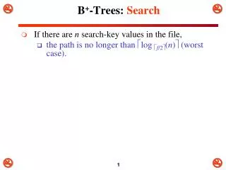
1. B+-Trees: Search • If there are n search-key values in the file, • the path is no longer than log f/2(n) (worst case).

2. External Sort-Merge • Sorting phase: • Sorts nB pages at a time • nB = # of main memory pages buffer • creates nR = b/nBinitialsorted runs on disk • b = # of file blocks (pages) to be sorted • Sorting Cost = read b blocks + write b blocks = 2 b

3. External Sort-Merge • Merging phase: • The sorted runs are merged during one or more passes. • The degree of merging (dM) is the number of runs that can be merged in each pass. • dM = Min (nB-1, nR) • nP = (logdM(nR)) • nP: number of passes. • In each pass, • One buffer block is needed to hold one block from each of the runs being merged, and • One block is needed for containing one block of the merged result.

4. External Sort-Merge • Degree of merging (dM) • # of runs that can be merged together in each pass = min (nB - 1, nR) • Number of passes nP = (logdM(nR)) • In our example • dM = 4 (four-way merging) • min (nB-1, nR) = min(5-1, 205) = 4 • Number of passes nP = (logdM(nR)) = (log4(205)) = 4 • First pass: • 205 initial sorted runs would be merged into 52 sorted runs • Second pass: • 52 sorted runs would be merged into 13 • Third pass: • 13 sorted runs would be merged into 4 • Fourth pass: • 4 sorted runs would be merged into 1

5. External Sort-Merge • External Sort-Merge: Cost Analysis • Disk accesses for initial run creation (sort phase) as well as in eachmergepass is 2b • reads every block once and writes it out once • Initial # of runs is nR = b/nB and # of runs decreases by a factor of nB - 1 in each merge pass, then the total # of merge passes is np = logdM(nR) • In general, the cost performance of Merge-Sort is • Cost = sort cost + merge cost • Cost = 2b + 2b * np • Cost = 2b + 2b * logdM nR • =2b(logdM(nR) + 1)

6. Catalog Information • Attribute • d: # of distinct values of an attribute • sl (selectivity): • the ratio of the # of records satisfying the condition to the total # of records in the file. • s (selection cardinality) = sl * r • average # of records that will satisfy an equality condition on the attribute • For a key attribute: • d = r, sl = 1/r, s = 1 • For a nonkey attribute: • assuming that d distinct values are uniformly distributed among the records • the estimated sl = 1/d, s = r/d

7. Using Selectivity and Cost Estimates in Query Optimization • Examples of Cost Functions for SELECT • S1. Linear search (brute force) approach • CS1a = b; • For an equality condition on a key, CS1a = (b/2) if the record is found; otherwise CS1a = b. • S2. Binary search: • CS2 = log2b + (s/bfr) –1 • For an equality condition on a unique (key) attribute, CS2 =log2b • S3. Using a primary index (S3a) or hash key (S3b) to retrieve a single record • CS3a = x + 1; CS3b = 1 for static or linear hashing; • CS3b = 1 for extendible hashing;

8. Using Selectivity and Cost Estimates in Query Optimization • Examples of Cost Functions for SELECT (contd.) • S4. Using an ordering index to retrieve multiple records: • For the comparison condition on a key field with an ordering index, CS4 = x + (b/2) • S5. Using a clustering index to retrieve multiple records: • CS5 = x + ┌ (s/bfr) ┐ • S6. Using a secondary (B+-tree) index: • For an equality comparison, CS6a = x + s; • For an comparison condition such as >, <, >=, or <=, • CS6a = x + (bI1/2) + (r/2)

9. Using Selectivity and Cost Estimates in Query Optimization • Examples of Cost Functions for SELECT (contd.) • S7. Conjunctive selection: • Use either S1 or one of the methods S2 to S6 to solve. • For the latter case, use one condition to retrieve the records and then check in the memory buffer whether each retrieved record satisfies the remaining conditions in the conjunction. • S8. Conjunctive selection using a composite index: • Same as S3a, S5 or S6a, depending on the type of index.