Exploring Genomes: Genes, Splice Variants, and Evolution
340 likes | 394 Vues
Understand genome databases, gene finding, ESTs, RefSeq, gene prediction, and codon usage to analyze genes, splice variants, and genomics evolution in eukaryotes and prokaryotes.

Exploring Genomes: Genes, Splice Variants, and Evolution
E N D
Presentation Transcript
Genome On Line Database (GOLD) • 243 Published complete genomes • 536 Prokaryotic ongoing genomes • 434 Eukaryotic ongoing genomes December 2004 : 1245 genome projects
Common Genome Browsers NCBI: http://www.ncbi.nlm.nih.gov/mapview/static/MVstart.html Eukaryote Only UCSC: http://genome.ucsc.edu Ensembl: http://www.ensembl.org Prokaryote Only MGV: http://cmbipc49.cmbi.kun.nl/genome/ TIGR: http://www.tigr.org/tigr-scripts/CMR2/CMRHomePage.spl /
What can we learn from genomes • Genes • Splice variants • Variation analysis • Promoters • Comparative Genomics • Evolution
5’UTR 3’UTR CDS
Looking for genes in genomes • Existing mRNA and EST data • Gene prediction program • Comparative genomics
ESTs (Expressed Sequence Tags) • cDNA provide a best tool to identify genes in a genome. • For unsequenced genomes it was the primary source for identifying genes • Basic strategy - select cDNA clones at random and perform a single automated read from one/both ends of the transcript. • Many clones will be redundant. • Very cost effective. • ESTs are short (400-600b), relatively inaccurate (2% error). • ESTs are correlated to known genes using a relatively small region of sequence alignment. • Used to discover genes, alternative splicing variants, etc.
Problems with ESTs -Incomplete Coverage Bias for high copy number genes -Experimental mistakes- not always reliable -Enrichment of 3’ ends of genes -High representation of cancer cells Usage of EST -Predicting of coding regions -Detecting of alternative splicing -Clustering to form genes
RefSeq database (NCBI) • The Reference Sequence (RefSeq) collection aims to provide a comprehensive, integrated, non-redundant set of sequences, including genomic DNA, transcript (RNA), and protein products, for major research organisms. • RefSeq standards serve as the basis for medical, functional, and diversity studies; they provide a stable reference for gene identification and characterization, mutation analysis, expression studies, polymorphism discovery, and comparative analyses.
Gene Finding Approaches • Learn characteristics of known genes • Search for new genes using characteristics • Different types of genes have different characteristics. • Prediction Status • The problem of gene prediction is very much open even in well studied genomes: • The number of genes in human keeps changing.
Gene Finding • Input • Chromosomal genetic sequence • Output • Region which encodes for gene • Strand and reading frame • Start and end of coding sequence • Exon-intron boundaries
Prokaryotes Vs. Eukaryotes Require different gene finding strategies. • Prokaryotes: • the genome is compact (Shorter intergenic regions, no introns). • several genes may reside on the same mRNA in different reading frames. • Promoter regions are more conserved. • Eukaryotes • large genomes; intron/exon structure; alternative splicing; pseudogenes, very long intergenic regions • The human genome: average gene ~ 27,800b. 8 exon ~ 100b. intron 100-30,000 b.
ORF Finding Open Reading Frames – sequences that presumably code for proteins. How can ORFs be detected? • All reading frames are checked. • Search for initiation and termination codons within a sequence. • Are these codons totally conserved? http://www.ncbi.nlm.nih.gov/gorf/gorf.html
Protein-coding Gene Characteristic • GC Content • Uneven codon usage • Amino acid bias • Species’ preferred codons • Promoter and splicing signals • These characteristics may aid in • Prediction. • Validation.
Codon Usage • DNA is not a random choice of possible codons for each amino acid. • It is an ordered list of codons that reflects evolutionary origin and constraints related to gene expression. • Each species has its own coding preferences – codon usage.
Codon Usage Database http://www.kazusa.or.jp/codon/ This site provides: • Codon usage tables per organism • Computation of codon usage for query coding sequences.
Codon Usage Preferences • Different codon usage for highly vs. weakly expressed genes. • in E. Coli genes were divided into 3 groups based on their codon usage – - regular genes (70%) - highly expressed genes (15%)- horizontally transferred genes (15%) • There is strong preferences in ORFs for specific codon pairs and for specific codons near terminators. • The base in the third position in each codon tends to repeat itself in the same ORF.
Sequence Signals • Prokaryotes: • Promoter (-35, -10 from TSS) • Ribosome Binding Site (Shine-Dalgarno) is conserved. Located ~ -15 upstream AUG. • Eukaryotes • Transcription signals TATA (~-30 TSS), cap signal, poly-adenylation site. Any signal may be missing. • Translation signalsKozak signal (immediately upstream ATG). • Splicing signals – recognized by the Spliceosome. Introns usually start with GT and end with AG.
Computational Approaches to Prediction • Various computational methods including decision trees, neural nets, Markov models and Hidden Markov models (HMM). • A model is studied based on known genes, and then applied to genomic sequences. • Each genome defines its own model.
Markov Models • Probabilistic approach. • Modeled by states and the probability of transition from one state to the next. • The probability of being at state X in step i depends only on the state we reached at step i-1. It has been found that ORFs have a reading-frame specific hexamer (6mer) composition. => the probability of the 6th base can be computed using the previous 5.=> The probability that a sequence is an ORF in a specific reading frame can be computed from its 6th-mer composition.
Grail II for finding Exons(Neural Network) Score of 6mers Score of 6mers in flanking region Markov model score GC composition Exon score GC composition in flanking Score for splicing acceptor output Score for splicing donor Hidden layer Input layer
GenScan (HMM) • One of most accurate programs • Best for human/vertebrate sequences • Markov parameters for different regions • Introns beginning at 3 phases • Exons: first, intermediate, last • Promoter region • 3’ and 5’ untranslated regions • Intragenic regions
The General Scheme • Obtain new genomic DNA sequence. • i. Translate in all 6 reading frames and compare to protein databases.ii. Perform database similarity search of expressed sequence tags (EST) database of same organism, or cDNA sequences if available. 3. Use gene prediction program to locate genes. 4. Analyze regulatory sequences and signals in the gene. Can help characterize putative genes.
Other gene Finding Tools • GeneMark (prokaryote, eukaryote) • http://opal.biology.gatech.edu/GeneMark/ • Glimmer (bacteria, archaea) • http://www.tigr.org/software/glimmer/ • GeneFinder (human, mouse, arabidopsis) • http://argon.cshl.org/genefinder/ • HMMgene (vertebrate, C. elegans) • http://www.cbs.dtu.dk/services/HMMgene/ http://www.tigr.org/genefinding/software.shtml
Prediction Evaluation Prediction tools are compared using two criteria: • Sensitivity - % true predicted genes out of the true genes in the genome. TP /(TP+FN) • Specificity - % true predicted non genes out of the total number of non genes. TN /(TN+FP) Both need to be high, results vary from genome to genome Accuracy comparisons tested on vertebrates SN SP GENSCAN 0.93 0.93 GRAILII 0.72 0.84
Functional RNA Genes • RNA genes are transcribed but are not translated – no codon preference exists.How can rRNA, tRNA and small RNA genes be predicted? • Promoter regions can be characterized, but remain a big challenge. • RNA secondary structure is important.Can be predicted using RNA structure prediction tools (MFOLD tool).
Comparative genomics • Finding Orthologs • Looking for genes in one species not found in another • Searching for conserved regulatory elements • Gene Clusters • Conserved regulatory networks
Conservation of the IGFALS (Insulin-like growth factor) Between human and mouse.