Capacitance Calculations using Method of Moments
570 likes | 661 Vues
Learn how the Method of Moments accurately calculates capacitance, using known charges to determine potentials. Developed by Ken Mei in 1962, this technique aids in determining capacitance for various geometries, aiding in EM applications.

Capacitance Calculations using Method of Moments
E N D
Presentation Transcript
Capacitance method of moments
Q a Capacitance of hollow sphere
Capacitance of a circular disk r R Voltage at origin = 0 a 2 -
Capacitance of a circular disk r a R 2 - Charge density is uniform s0
Capacitance of a circular disk r a R 2 - Charge density decreases s0(1-r/a)
This technique was developed in a Ph.D. thesis by Ken Mei in 1962. His adviser was Jean van Bladel.
Method of moments • a known charge causes a potential • what is the potential? • a measured or known potential is caused by an unknown charge • what was that charge? • used in em to find current distributions on antennas, scattering objects such as cubes, sleds, planes, and missles • PhD theses, faculty publications
V(a) V(b) Q2 Q1 2 equations 2 unknowns
V(a) V(b) Q2 Q1
>> A = [1/4 1/5 ; 1/5 1/4] ; >> V = [1 ; 1] ; >> Q = V’ / A % ‘transpose Q = 2.2222 2.2222 >> QQ = A \ V; QQ = 2.2222 2.2222
complications??? r1 r2 • The potential @ each charge sphere is specified as V1 or V2 • Locations are with respect to an origin.
solution to singularity Assume that the potential is uniform within the sphere and it is equal to the value at its edge r = a.
1 1 1 1 1 1
Q = • 4.69 2.56 4.69 -4.69 -2.56 -4.69 • >>
a b -a -a a -b -b b Capacitor C = Q / V rj ri
b -b -b b Capacitor C = Q / V Harrington – p. 27 Dwight 200.01 & 731.2
b -b -b b Capacitor C = Q / V
MATLAB • clear; clf; • N=9; • az=37.5; • el=5;
%identify subareas • for m = 1:2 • for h = 1:N • for k = 1:N • a(m - 1)*N*N + (h - 1)*N + k, :)=[m, h, k]; • end • end • end
%calculate matrix elements • for h=1:2*N*N • for k=1:2*N*N • aa=norm(a(h, :) - a(k, :)); • if aa==0 • b(h, k) = 2 * sqrt(pi); • else • b(h, k) =1 / aa; • end • end • end
%set voltages on plates • for h=1:N*N • V(h) = +1/2; • V(h+N*N) = -1/2; • end
%calculate charges • Q = V*inv(b); • %top plate • QA(1:N*N) = Q(1:N*N); • %bottom plate • QB(1:N*N)=Q(N*N+1:2*N*N);
%plot • [x,y]=meshgrid(1:N); • for i=1:N • za(1:N,i)=QA((i-1)*N+1:(i-1)*N+N)'; • zb(1:N,i)=QB((i-1)*N+1:(i-1)*N+N)'; • end • mesh(x,y,za) • hold on • mesh(x,y,zb)
QT=0; for j=1:N*N QT=QT+Q(j); end QT
What have you done? You have learned a technique, to accurately calculate the capacitance of a parallel plate capacitor! Big deal!
Capacitance of a circular disk r a R 2 - Charge density is uniform s0
Capacitance of a circular disk r a R 2 - Charge density is noniform
C = 3.9420 C = 3.2367 C = 2.7026 C = 3.6332
capacitance of a unit cube Hwang & Mascogni – “Electrical capacitance of a unit cube” – Journal of Applied Physics 3798-3802 (2004).
2a C a
note the charge density at the corner
a h Sava V. Savov February 1, 2004
1 2 3 x. • E = s /2 • V = x s /2 • V1 = 2 [0/2 s1 + 1 s2 + 2/2 s3 ] • V2 = 2 [1/2 s1 + 0 s2 + 1/2 s3] • V3 = 2 [2/2 s1 + 1 s2 + 0/2 s3]
1 2 3 • V1 0 1 2/2 s1 • V2 = 2 1/2 0 1/2 s2 • V3 2/2 1 0 s3 • pn junction • double layer • VLSI
pn junction • linear quadratic • V[-2d] - 0.36 - 2 • V[-d] - 0.18 - 3/2 • V[0] = 0 or 0 • V[d] + 0.18 + 3/2 • V[2d] + 0.36 + 2
matrix • 0 1 2 3 4/2 • 1/2 0 1 2 3/2 • 2/2 1 0 1 2/2 • 3/2 2 1 0 1/2 • 42 3 2 1 0
MATLAB • [V] = [matrix] [Q] V V r r x x
Calculate vector “V” • clear • clf • m=input('What is the size of the matrix? ...'); • for i=1:m • v(i)=NaN; • end • v
Calculate matrix “a” • for i=1:m • for j=1:m • a(i,j)=NaN; • end • end
for i=1:m • for j=i:m • if i==j • a(i,j)=0; • b(i)=i; • elseif i<j & j<m a(i,j)=(j-b(i)); elseif i<j & j==m • a(i,j)=(j-b(i))/2; • end • end • end