Download

1 / 75
760 likes | 969 Vues
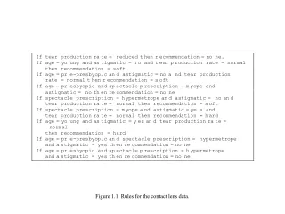
Figure 1.1 Rules for the contact lens data. Figure 1.2 Decision tree for the contact lens data. (a). (b). Figure 1.3 Decision trees for the labor negotiations data. Figure 2.1 A family tree and two ways of expressing the sister-of relation. Figure 2.2 ARFF file for the weather data.

E N D
(a) (b) Figure 1.3 Decision trees for the labor negotiations data.
Figure 2.1 A family tree and two ways of expressing the sister-of relation.
If x=1 and y=0 then class = a If x=0 and y=1 then class = a If x=0 and y=0 then class = b If x=1 and y=1 then class = b Figure 3.2 The exclusive-or problem.
If x=1 and y=1 then class = a If z=1 and w=1 then class = a Otherwise class = b Figure 3.3 Decision tree with a replicated subtree.
Default: Iris-setosa 1 • except if petal-length 2.45 and petal-length < 5.355 2 • and petal-width < 1.75 3 • then Iris-versicolor 4 • except if petal-length 4.95 and petal-width < 1.55 5 • then Iris-virginica 6 • else if sepal-length < 4.95 and sepal-width 2.45 7 • then Iris-virginica 8 • else if petal-length 3.35 9 • then Iris-virginica 10 • except if petal-length < 4.85 and sepal-length < 5.95 11 • then Iris-versicolor 12 Figure 3.4 Rules for the Iris data.
Shaded: standing Unshaded: lying Figure 3.5 The shapes problem.
PRP = - 56.1 + 0.049 MYCT + 0.015 MMIN + 0.006 MMAX + 0.630 CACH - 0.270 CHMIN + 1.46 CHMAX Figure 3.6(a) Models for the CPU performance data: linear regression.
Figure 3.6(b) Models for the CPU performance data: regression tree.
Figure 3.6(c) Models for the CPU performance data: model tree.
(a) (b) (c) (d) Figure 3.7 Different ways of partitioning the instance space.
(a) (b) (c) 1 2 3 a 0.4 0.1 0.5 b 0.1 0.8 0.1 c 0.3 0.3 0.4 d 0.1 0.1 0.8 e 0.4 0.2 0.4 f 0.1 0.4 0.5 g 0.7 0.2 0.1 h 0.5 0.4 0.1 … (d) Figure 3.8 Different ways of representing clusters.
(a) (b) Figure 4.2 Tree stumps for the weather data. (c) (d)
(a) (b) (c) Figure 4.3 Expanded tree stumps for the weather data.
(a) (b) Figure 4.6 (a) Operation of a covering algorithm; (b) decision tree for the same problem.
Figure 4.7 The instance space during operation of a covering algorithm.
(a) (b) Figure 6.1 Example of subtree raising, where node C is “raised” to subsume node B.
p number of instances of that class that the rule selects; • t total number of instances that the rule selects; • p total number of instances of that class in the dataset; • t total number of instances in the dataset. Figure 6.4 Definitions for deriving the probability measure.
Figure 6.5 Algorithm for forming rules by incremental reduced error pruning.
Figure 6.6 Algorithm for expanding examples into a partial tree.
(a) (c) (b) Figure 6.7 Example of building a partial tree.
(d) (e) Figure 6.7 (continued) Example of building a partial tree.
Exceptions are represented as Dotted paths, alternatives as solid ones. Figure 6.8 Rules with exceptions, for the Iris data.
Figure 6.12 Model tree for a dataset with nominal attributes.
(a) (b) (c) Figure 6.13 Clustering the weather data.
(d) (e) Figure 6.13 (continued) Clustering the weather data.
(f) Figure 6.13 (continued) Clustering the weather data.
(a) Figure 6.14 Hierarchical clusterings of the Iris data.
(b) Figure 6.14 (continued) Hierarchical clusterings of the Iris data.
data A 51A 43B 62B 64A 45A 42A 46A 45A 45 B 62A 47A 52B 64A 51B 65A 48A 49 A 46 B 64A 51A 52B 62A 49A 48B 62A 43A 40 A 48B 64A 51B 63A 43B 65B 66 B 65A 46 A 39B 62B 64A 52B 63B 64A 48B 64A 48 A 51A 48B 64A 42A 48A 41 model A=50, A =5, pA=0.6 B=65, B =2, pB=0.4 Figure 6.15 A two-calss mixture model.
Figure 7.2 Discretizing temperature using the entropy method.
64 65 68 69 70 71 72 75 80 81 83 85 no yes yes no yes yes yes no no yes yes no yes yes F E D C B A 66.5 70.5 73.5 77.5 80.5 84 Figure 7.3 The result of discretizing temperature.
Figure 7.4 Class distribution for a two-class, two-attribute problem.
Figure 7.5 Number of international phone calls from Belgium, 1950–1973.