Download
1 / 39
400 likes | 610 Vues
J Q konv (x+ D x). x. T mi. x+ D x. Reaktorwand. Kühlmantel. x. T ma. J Q über (x). J Q konv (x). T. 3. Macroscopic transport processes : Heat and mass transfer in presence of convection 3.1 Heat transfer in technical appliances

E N D
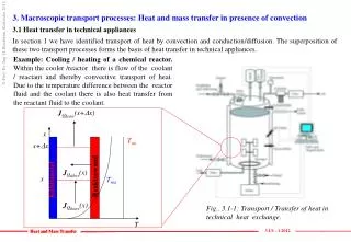
JQkonv(x+Dx) x Tmi x+Dx Reaktorwand Kühlmantel x Tma JQüber(x) JQkonv(x) T 3. Macroscopictransportprocesses: Heatandmasstransfer in presenceofconvection 3.1 Heattransfer in technicalappliances In section 1 wehaveidentifiedtransport of heatbyconvectionandconduction/diffusion. The superposition of thesetwotransportprocessesforms the basis of heattransfer in technicalappliances. Example: Cooling / heating of a chemical reactor. Within the cooler /reactor there is flow of the coolant / reactant and thereby convective transport of heat. Due to the temperature difference between the reactor fluid and the coolant there is also heat transfer from the reactant fluid to the coolant. Fig.. 3.1-1: Transport / Transfer of heat in technical heat exchange. 3.1/1 - 1.2012
Temperatur Radius The heat flux from the reactant to the coolant occurs via conduction of heat through the reactor wall and the adjacent boundary layers of the fluids at rest. Therefore, heat transfer in any case is based on heat conduction! Convection only modifies the boun-dary conditions. Heat transfer is a boundary value problem of convective / diffusive transport of heat. 3.2 General model for heat transfer From the discussion in section 2 we have learned to write any heat transfer problem as: As heat transfer occurs by heat conduction through the wall boundary layer we can write for the heat flux: From that we obtain for the heat transfer coefficient: For few problems in section 2 the temperature gradient could be accessed analytically. Tmi TWi Medium 2 Medium 1 TWa Tma Ri Ra Fig. 3.1-1: Heat transfer as heat conduction through a layered geometry. Fig. 3.2-1: General model for heat transfer. In most technical appliances velocity- and temperature fields cannot be calculated in a simple way (as in the examples in section 2.) so that the temperature gradient (dT/dy)y=0 has to be approximated. In these cases a linearization of the temperature near the wall (system boundary) is applied (Taylor-series of temperature, see figure 3.2-1): With DT = T0 – TW we obtain: 3.2/1 - 1.2012
According to the model the heat transfer coefficient a is the heat conductivity l divided by the thickness Dy of a fictitious temperature boundary layer which results from the linearization of the temperature. The problem of the unknown heat transfer coefficient a is now shifted to the fictitious boundary layer thickness Dy. The determination of this is done mostly by experiments resulting in correlations for the heat transfer coefficients for the various arrangements. Correlations for heat transfer coefficients. Correla-tions for heat transfer coefficients are generally given in the form: For simple problems (heat transfer from a sphere into a fluid at rest, cold bridge, non stationary heating etc. ) correlations of the kind of equation (3.2-6) can be accessed analytically. For the more complicated technical cases the correlations have to be developed from experimental investigations. Fig. 3.2-2: Nusselt number for laminar flow in tubes. Laminar flow in tubes. Equation (3.2-7) exhibits that the (lenght averaged) Nusselt number asymptotically approaches a value of 3,66 for long tubes (thermal upgrowth). 3.2/2 - 1.2012
Turbulent flow in tubes. with Fig.. 3.2-3 a, b: Nusselt number for turbulent flow in tubes. The dependence of Nu on Re in turbulent flow is considerably larger than in laminar flow; Nu decreases with increasing lenght of tube; influence of Prandtl number stronger than in laminar flow. 3.2/3 - 1.2012
Tabl. 3.2-1: Correlations for the Nusselt number for different arrangements (further information in literature (e.g. VDI-Wärmeatlas). 3.2/4 - 1.2012
Medium 1 Medium 2 3.3 Heat transfer in technical heat exchangers 3.3.1 Over all heat transfer coefficient In section 3.2 we have discussed heat transfer from a fluid to a wall (to the system boundary). In technical heat exchangers we find a) transfer of heat from a fluid to the wall, b) transfer of heat through the wall and c) transfer of heat from the wall to a fluid. In principle, we have a series of heat resistances formed by a boundary layer, the wall and a second boundary layer. The problem of heat resistances in series has been discussed in detail in section 2.1.4. This has to be transferred now to heat transfer in technical heat exchangers, see figure 3.3.1-1. In figure 3.1-1 we have a technical heat exchanger. In the inner tubes a hot gas flow from the bottom to the top is established (e.g. hot reaction products from a high temperature reaction). In the annuli around the inner tubes coolant is coflowing (e.g. water which is vaporized when flowing from the bottom to the top). Due to the temperure differences between the hot gas flow (medium 1) and the coolant (medium 2) we have temperature gradients perpendicular to the direction of the flow. This temperature gradient is the driving force for heat transfer from the hot to the cool (from medium 1 to medium 2). The temperature profile across a tube in the heat exchanger is enlarged in Fig. 3.3.1-2 Fig. 3.3.1-1: Example for a technical heat exchanger. 3.3.1/1 - 1.2012
s1 s2 Tmi T TWi Temperatur Medium 2 Medium 1 TWa Tma A Radius JQ JQ JQ l1 l2 x s2 T1 T1/2 T2/3 Ri Ra T3 Fig. 3.3.1-2: Temperature profile across a tube in the heat exhanger. l3 The temperature profile in figure 3.3.1-2 across a tube in the heat exchanger resembles the temperature profile in a layered material, see section 2.1.4, when replacing the two outer layers by fluid boundary layers. This problem has been treated as a heat conduction problem through heat conduction resistances in series, see fig. 3.3.1-3. For this problem we have derived: with: Fig. 3.3.1-3: Heat transfer in a layered material by heat conduction. For the over all heat transfer coefficient we have: ki:heat conductivities per length, 1/ki: resistance. The reciprocals of the heat transfer coefficients are lenght-specific resistances wich add for the heat transfer through all layers. 3.3.1/2 - 1.2012
Temperatur Medium 2 Medium 1 Tmi TWi TWa Radius Tma Ri Ra Fig. 3.3.1-4: Temperature profile across a tube in the heat exhanger. For the heat exchanger indicated in figure 3.3.1-2 the single outer layers are replaced by the temperature boundary layers (see figure 3.3.1-4). From this we obtain: Internal side: Wall: External side Resolving equations (3.5.1-4) to (3.5.1-6) for the temperature differences and adding we obtain: Transformation with Aa~AW~Ai=A gives: According to equation (3.3.1-8) the heat flux by heat transfer is proportional to the area and the total temperature difference. Proportionality factor is the over all heat transfer coefficient. (All quantities are local quantities, i.e. dependent on the coordinate in flow direction.) 3.3.1/3 - 1.2012
3.3.2 Simple heat transfer problems from process engineering In the previous section we have derived the basic equation for heat transfer with This equation will be used in the following to treat some simple heat transfer problems from process engineering. Temperature profile in the coolant for a well stirred tank reactor. In the reactor an exothermic chemical reaction is performed at a constant temperature Tmi. To keep temperature at constant the heat of reaction has to be transferred to the coolant. The temperature inside the reactor is homogeneous, i.e. constant everywhere inside the reactor. This is achieved by intensively stirring the reactor. We look for the temperature profile in the coolant, the effectivity of the heat exchanger, the transferred heat per time… Fig. 3.3.2-1: Heat transfer in a chemical reactor (well stirred tank reactor). 3.3.2/1 - 1.2012
x Tmi Reaktorwand Kühlmantel Tma JQkonv(x+Dx) T JQüber(x) JQkonv(x) Temperature profile. For the determination of the temperature within the coolant we use a simple heat balance for a differential balance volume as indicated in figure 3.3.2-2. The heat balance according to fig 3.3.2-2 gives: with (T=Tma), convective fluxes according to page 1.3.1/1 we obtain: Balance: Linearization of temperature (taylor series) gives: Using this in the heat balance and separation of variables and using dT = d(Tmi-T) results in: x+Dx x Fig. 3.3.2-2: Heat balance for calculation of the temperature profile in the coolant (heat conduction in flow direction neglected!). Solution of this ordinary differential equation: Boundary condition: T=T0 for A=0, then C = ln(Tmi-T0). 3.3.2/2 - 1.2012
JQkonv(x+Dx) x Tmi x+Dx Reaktorwand Kühlmantel x Tma T JQüber(x) JQkonv(x) Further: The solution then is: According to equation (3.3.2-12) the temperature difference Tma-T exponentially approaches zero. Generally the temperature profile in heat exchangers is written in the form: Effectivity.g is the effectivity of the heat exchanger.g describes the approach to thermal equilibrium. For the heat exchanger under consideration for g = 1 the maximum possible heat is transferred. Transformation of equation (3.3.2-12) gives: Fig. 3.3.2-3: Temperature profile in the coolant. 3.3.2/3 - 1.2012
1-1/e=0,63 The ratio is called number of transfer units. NTU can be interpreted as the ratio of heat flux per Kelvin by heat transfer to the heat flux per Kelvin by convection. The larger NTU the more effective the heat exchanger works. From equation (3.3.2-14) for NTU = 1 follows: One tranfser unit causes a 63% approach to thermal equilibrium for this kind of heat exchanger, compare figure 3.3.2-3. The number of transfer units can be tuned by the over all heat transfer coefficient, the area of the heat exchanger, the mass flux and the specific heat of the coolant! Fig. 3.3.2-3: Temperature profile in the coolant. Total heat flux for the heat exchanger. The total heat flux of the heat exchanger can be calculated easily with the help of the basic equation for heat transfer: In equation (3.3.2-17) Tm is a temperature averaged over the area of the heat exchanger that causes the identical total heat flus as the factual temperature profile in the coolant. 3.3.2/4 - 1.2012
Fig. 3.3.2-3: Temperature profile in the coolant. The averaged temperature Tm is calculated with the help of a total heat balance for the heat exchanger: This heat flux has to be absorbed from the coolant: Comparing equations (3.3.2-18) and (3.3.2-19) we obtain: Transformation gives: Taking NTU from (3.3.2-12) yields: For this kind of heat exchanger the total heat flux can be easily calculated using equation (3.3.2-18) using an averaged temperature difference which is given by the „logarithmic mean“ according to equation (3.3.2-22). This logarithmic mean is smaller than the arithmetic mean due to the exponential decay of the temperature difference, see figure 3.3.2-3. 3.3.2/5 - 1.2012
T Innenrohr Tma Außenrohr x x JQkonv(x+Dx) JQkonv(x+Dx) JQüber(x) JQkonv(x) JQkonv(x) Tmi Temperature profiles in a heat exchanger with coflow. We treat a simple heat exchanger with coflowing coolant and hot flow, compare figure 3.3.2-4. In the inner tubes a hot flow is flowing from the bottom to the top. In the annuli around the inner tubes a coolant is co-flowing. We calculate the temperatures in the hot and cold flow, the efficiency and the total heat flux. Temperatuer profiles. For the determination of the temperatures we perform a simple heat balance for a differential balance volume of the heat exchanger, compare figure 3.3.2-4. Heat balance for the coolant: With convective heat fluxes according to section 1.3.1 and the basic heat transfer equation we obtain: x x+Dx Fig. 3.3.2-4: Heat balance for calculation of the temperature profiles in a coflowing heat exchanger. Balance: The balance contains Tmaand DT= Tmi-Tma, therefore determination of DT(x) First! 3.3.2/6 - 1.2012
T Innenrohr Tma Außenrohr x x x x+Dx JQkonv(x+Dx) JQkonv(x+Dx) JQüber(x) JQkonv(x) JQkonv(x) Tmi Expanding temperature into a Taylor-series and linearization: Introducing into the heat balance gives: Analogously we obtain the balance for the hot flow: Solving equations (3.3.2-29) and (3.3.2-31) for the temperature gradients and subtracting gives: Noting the definition of the temperature difference Fig. 3.3.2-5: Heat balance for calculation of the temperature profiles in a coflowing heat exchanger. We obtain finally a differential equation for the temperature difference DT: This differential equation can be solved easily after separation of variables. 3.3.2/7- 1.2012
Integration gives: If the remaining integral on the right hand side is replaced with the help of the averaged total heat transfer coefficient we obtain: Resolving the logaritm we obtain: The temperature difference in the heat exchanger exponentially decreases! Equation (3.2.2-38) can be transformed using dA = Agesdx into: With that solution for the temperature difference the temperatures in the coolant and the hot flow can be calculated. For that we use equations (3.3.2-29) and (3.3.2-31) after transformation: Using DT from equation (3.3.2-39) we obtain: 3.3.2/8- 1.2012
Solution for the temperature in the hot flow: Solution for the temperature in the coolant: The solution for the temperature in the coolant according to equation (3.3.2-45) is the effectivity g of the heat exchanger in coflow! Equation (3.3.2-44) can be rewritten as: Fig. 3.3.2-6: Effectivity of a coflow heat exchanger according to equation (3.3.2-45), (NTUi = 5). Fig. 3.3.2-7: Temperatur profiles in the coflow heat exchanger according to equation (3.3.2-44a), (NTUi =5). 3.3.2/9- 1.2012
Fig. 3.3.2-7: Temperature profiles in the coflow heat exchanger. Total heat flux in coflow heat exchanger. Equation (3.3.2-34) can be transformed by separating variables: or Integrating and replacing the term in brackets of equation (3.3.2-46) by (NTUi + NTUa) from equation (3.3.2-37) and using dJQ=kDTdA, we obtain: Comparing this with the general equation for heat transfer we obviously and advantageously introduce again a „logarithmic mean“ for calculation of the total heat flux in this kind of heat exchanger. 3.3.2/10- 1.2012
T Innenrohr JQkonv(x+Dx) Außenrohr x x Tma Tmi JQkonv(x+Dx) JQüber(x) JQkonv(x) JQkonv(x) Temperature profiles in a counter-flow heat exchanger. We treat a simple heat exchanger with counter flowing coolant and hot flow, compare figure 3.3.2-8. In the inner tubes a hot flow is flowing from the right to the left. In the outer flow a coolant is counter–flowing flowing from left to right. We calculate the temperatures in the hot and cold flow, the efficiency and the total heat flux. Temperature profiles. For the determination of the temperatures we perform again a simple heat balance for a differential balance volume of the heat exchager, compare figure 3.3.2-8. Heat balance for the coolant (same as for the co-flowing heat exchanger): Balance equation again contains Tmaand DT= Tmi-Tma, therefore, first calculation of DT(x)! Heat balance for the hot medium: Same procedure as for the co-flowing heat exhanger (expansion of temperature into a Taylor series etc.) gives: x x+Dx Fig. 3.3.2-8: Heat balance for calculation of the temperature profiles in a counter flowing heat exchanger. Only difference to the co-flowing heat exchanger: sign in the heat balance ! 3.3.2/11 - 1.2008
T Innenrohr JQkonv(x+Dx) Außenrohr x x Tma Tmi x x+Dx Abb. 3.3.2-8: Wärmebilanz zur Berechnung des Temperaturverlaufs im Gegenstromwärmeübertrager. JQkonv(x+Dx) JQüber(x) JQkonv(x) JQkonv(x) Solving equations (3.3.2-52) and (3.3.2-53) for the temperature gradients and subtracting gives: Noting the definition of the temperature difference, we obtain finally a differential equation for DT: Solution after separation of variables gives: Factoring out (-1) and removing the logarithm gives: The temperature difference in the counter-flowing heat exchanger equally well decreases exponentially! However, in this case much lower ! Equation (3.3.2-58) with the help of dA = Agesdx can be rewritten as: 3.3.2/12 - 1.2008
With the solution for the total temperature difference DT the temperature profiles in the hot and cold flow can be calculated. For this we use equantion (3.3.2-51) and (3.3.2-53) which can be written as: Using DT from the equation (3.3.2-59) gives: Then the temperature in the hot flow using the boundary condition Tmi = Tmie forx=0 andDT0=Tmie-Tma0: For the temperature in the cold flow we obtain using the boundary condition Tma = Tmao for x = 0: In the equations for the temperatures in the hot and counter-flowing cold flow the yet unknown temperature Tmie is containe, which must be calculated first. For that we use equation (3.3.2-64) for x=1 and add (Tma0-Tma0). Transformation then results in: If this result is substituted in equation (3.3.2-65) we obtain an expression for the effectivity g of the counter flowing heat exchanger. 3.3.2/13 - 1.2008
Using equation (3.3.2-66) in equation (3.3.2-64) we obtain after addition of (Tmi0-Tmi0) and some transformations: Equation (3.3.2-68) can be rewritten as : The temperature profiles according to (3.3.2-68a) is given in figure 3.3.2-10. Fig. 3.3.2-9: Effectivity of a counter-flowing heat exchanger (NTUi = 5). 3.3.2/14 - 1.2008
Abb. 3.3.2-10: Temperature profile in a counter-flowing heat exchanger according to equation (3.5.2-68a) (NTUi = 5). 3.3.2/15 - 1.2008
Summary of section 3.1 to 3.3 • A general model forheattransferhasbeendiscussed. • Correlationsforheattransfercoefficientshavebeenintroduced. • Heattransferandover all heattransferhavebeenintroduced. • Some simple types of heatexchangershavebeentreated. • Temperatureprofiles in heatexchangers, effectivity of heatexchangersand total heatfluxes in heatexhangerscanbecalculated. 3.3.2/16- 1.2012
Jnikonv(x+Dx) Jnakonv(x+Dx) Jnüber(x) Jnikonv(x) Jnakonv(x) x 3.4 Mass transfer in technical appliances In section 1 we have identified transport of mass by convection and diffusion. The superposition of these two transport processes forms the basis of mass transfer in technical appliances. x+Dx x Example: Mass transfer in an absorption tower. Within the absorption tower there is flow of the solvent from top to bottom and of the gas from bottom to top and thereby convective transport of mass. Due to the concentration difference of the transferred chemical species between the gas and the solvent there is also mass transfer from the gas to the solvent. Fig. 3.4-1: Mass transfer in a technical absorption tower. 3.4/1 - 1.2012
ck0 y dD Dy ckW ck The mass flux from the gas to the solvent occurs via diffusion of mass through the phase boundary and the adjacent boundary layers. Therefore, mass transfer in any case is based on diffusion! Convection only modifies the boundary layer conditions. Mass transfer is a boundary value problem of convective / diffusive transport of mass. 3.4.1 General model for mass transfer From the discussion in section 2.5 we have learned to write any mass transfer problem as: As mass transfer occurs by diffusion through the phase boundary we can write for the mass (molar) flux: Comparing eq. (3.4.1-1) and (3.4.1-2) we obtain for the mass transfer coefficient: For few problems in section 2 the concentration gradient could be accessed analytically. Fig. 3.4.1-1: General model for mass transfer. In most technical appliances velocity- and con-centration fields cannot be calculated in a simple way (as in the examples in section 2.) so that the concen-tration gradient (dck/dy)y=0 has to be approximated. In these cases a linearization of the concentration near the phase boundary is applied (Taylor-series of concentration, see figure 3.4.1-1): With Dck = ckW – c k0 we obtain: 3.4.1/1 - 1.2012
According to the model the mass transfer coefficient b is the diffusion coefficient Dk divided by the thickness Dy of a fictitious concentration boundary layer which results from the linearization of the concentration profile. The problem of the unknown mass transfer coefficient b is now shifted to the fictitious boundary layer thickness Dy. The determination of this is done mostly by experiments resulting in correlations for the mass transfer coefficients for the various arrangements. Correlations for mass transfer coefficients. Correla-tions for mass transfer coefficients are generally given in the form: For simple problems (mass transfer from a sphere into a fluid at rest, diffusion into the pores of a catalyst etc.) correlations of the kind of equation (3.4.1-6) can be accessed analytically. For the more complicated technical cases the correlations have to be developed from experimental investigations. Laminar flow in around spheres. For mass transfer from spheres into a fluid at rest the Sherwood number is, similar as the Nusselt Number for heat transfer from a sphere, Sh=2. If there is laminar flow around the sphere the appropriate correlation is given by: Correlations for other cases relevant for process engineering are given in table 3.4.1-1. From the table the similarity of heat and mass transfer is obvious. 3.4.1/2 - 1.2012
Table. 3.4.1-1: Correlations for the Sherwood number for mass transfer in arrangements important in provess engineeerimng (more information e.g. M. Baerns et al.: Technische Chemie, M. Jischa: Konvektiver Impuls-, Wärme- und Stoffaustausch, E.U. Schlünder: Einführung in die Stoffübertragung, ). 3.4.1/3 - 1.2012
3.4.2 Over all mass transfer coefficient for mass transfer in technical appliances In section 3.4.12 we have discussed mass transfer from a fluid to a phase boundary. In technical mass exchangers we find a) transfer of mass from a fluid to the phase boundary, b) transfer of mass through the phase boundary and c) transfer of heat from the phase boundary to a second fluid. In principle, we have a series of mass transfer resistances formed by a boundary layer, the phase boundary and a second boundary layer. The problem of mass transfer resistances in series can be treated analogously to the problem of heat transfer resistances in series. This will be applied now to mass transfer in technical mass exchangers, see figure 3.4.2-1. In figure 3.4.2-1 we have a technical film absorption apparatus. The solvent enters at the top and moves via the different stages to the bottom. A gas phase is counter flowing from bottom to the top. A chemical component k, contained in the gas flow is transferred into the solvent. Due to the concentration differences of the component k between the gas flow (medium i) and the solvent (medium a) we have concentration gradients perpendicular to the direction of the flow. This concentration gradients are the driving forces for mass transfer from the gas to the solvent (from medium i to medium a). The concentration profile across a stage in the mass exchanger is enlarged in Fig. 3.4.2-2 Fig. 3.4.2-1: Example of a technical mass exchanger (film apsorption apparatus). 3.4.2/1 - 1.2012
ck Solvent cki ckPhi ckPha cka Gas x The molar flux from the bulk of the gas phase to the phase boundary is given according to the general mass transfer equation by: The molar flux from the phase boundary to the bulk of the solvent phase similarly is given by: If there is nor resistance for the transfer through the phase boundary then the concentrations left and right to the phase boundary ckPhiand ckPha are in phase equilibrium (for absorption Henry‘s law applies). Fig. 3.4.2-1: Example of a technical mass exchanger (film apsorption apparatus) and concentration profiles. 3.4.2/2 - 1.2012
ck Solvent cki ckPhi cki* ckPha cka Gas x Applying Henry‘s law we can write: and also Here c*ki is the concentration that would be in phase equilibrium with cka, compare figure 3.4.2-2. Assuming stationary conditions the molar fluxes according to equations (3.4.2-1) and (3.4.2-2) are equivalent. Resolving these equations for the concentration differences we obtain: Multiplying equation (3.4.2-6) by k*k, we obtain: or by using equations (3.4.2-3) and (3.4.2-4) Fig. 3.4.2-2: Concentration profiles for mass transfer from gas solvent. Adding equations (3.4.2-5) and (3.4.2-8) gives: and finally 3.4.2/3 - 1.2012
ck Solvent cki ckPhi cki* ckPha cka Gas x cka* We have now described the mass transfer analogously to heat transfer: The molar flux is proportional to the area, the over all mass transfer coefficient and a total concentration difference. The driving concentration difference has to be calculated somewhat differently compared to heat transfer. This difference is due to the concentration jump in the phase boundary. with In equations (3.4.2-10) and (3.4.2-11) the mass transfer has been formulated with the concentration in the gas phase. The same is possible with the concentrations in the liquid phase. From the analogous considerations we obtain equations (3.4.2-12) and (3.4.2-13). Fig. 3.4.2-3: Concentration profiles for mass transfer from gas solvent. 3.4.2/4 - 1.2012
3.4.3 Simple mass transfer problems from process engineering In the preceeding section the basic equations for mass transfer have been derived as: These relations now are to be used for the treatment of simple problems of mass transfer in process engineering. Concentration profiles in a technical mass transfer apparatus (absorption tower). In a technical absorption tower (compare figure 3.4.3-1) a chemical compound k in a gas mixture is transferred to a solvent. The gas mixture containing the component k enters the tower at the bottom and flows in upward direction. The solvent is added at the top of the tower and flows downwards. Requested is the concentration profile of the component k in the gas phase and the liquid phase. Fig. 3.4.3-1: Mass transfer within an absorption tower. 4.5.2/1 - 2.2008
Jnakonv(x+Dx) Jnikonv(x+Dx) Jnüber(x) ck ckio cki ckie ckie cka Jnakonv(x) Jnikonv(x) cka0 x x For calculation of the concentration profiles within the absorption tower a simple mass balance for the component k for a differential volume of the absorption tower is formulated, see figure 3.4.3-2. Balance of molar fluxes for the gas phase in the balance volume: Inflow = Outflow + Transfer For the molar fluxes we have: Balance: Epansion of the concentration into a Taylor-series and linearisation gives: x+Dx x Fig. 3.4.3-2: Material balance for a technical absorption tower and concentration profiles (schematically). 4.5.2/2 - 2.2008
x Jnikonv(x+Dx) Jnakonv(x+Dx) x+Dx x Jnüber(x) Jnikonv(x) Jnakonv(x) Inserting into the material balance gives: Here we have used : A = a . Ageo.Dx. The balance for the liquid phase gives analogously: Expansion of the concentration into a Taylor-series, linearisation and insertion into the balance equation gives: By use of We obtain from equation (4.5.2-15): Fig. 3.4.3-2: Material balance for a technical absorption tower. Adding equation (4.5.2-11) and (4.5.2-17) gives: From the definition of the over all mass transfer coefficient from equation (4.5.2-2) and (4.5.2-4) follows: 4.5.2/3 - 2.2008
x Jnikonv(x+Dx) Jnakonv(x+Dx) x+Dx x Jnüber(x) Jnikonv(x) Jnakonv(x) Finally after transformation and separation of variables we have: Integration gives: For the integral on the right hand side one can write analogously as in the calculation of the temperature profiles in heat exchangers: With this we obtain analogously to the profile of the temperature differences in counter-flow heat exchangers: After removing the logarithm follows: Fig. 3.4.3-2: Material balance for a technical absorption tower. The concentration difference between the concentration of the component k in the gas phase and the concentration in the liquid phase decreases exponentially (compare counter-flow heat exchanger). A similar result will be obtained, if the mass transfer is formulated with the concentration of the liquid phase (equations 4.5.2-3 and 4.5.2-4). 4.5.2/4 - 2.2008
With the solution for the concentration difference it is possible to determine the concentration profiles in the liquid phase and the gas phase. For that we use equation (4.5.2-11) and equation (4.5.2-15), respectively. Inserting the solution from equation (4.3-24) and integrating gives: Similarly we obtain for the liquid phase (equation (4.5.2-15)): The concentration ck*io is the concentration which is in thermodynamic equilibrium with the concentration ckae, compare equation (4.5.2-16). This concentration is not yet known and must be determined (compare counter-flow heat exchanger). For this equation (4.5.2-26) is formulated for the total tower height and resolved for the requested concentration difference. After some transformations we obtain: The concentration profiles of the component k in the gas phase and the liquid phase as well as the concentration difference are plotte4d in figures 3.4.3-3 and 3.4.3-4. 4.5.2/5 - 2.2008
Fig. 3.4.3-3: Concentration difference in an absorption tower. Fig. 3.4.3-4: Concentration profiles in an absorption tower. 4.5.2/6 - 2.2008
Summary of section 3.4 • A general model formasstransferhasbeendiscussed. • Correlationsformasstransfercoefficientshavebeenintroduced. • Masstransferandover all masstransferhavebeenintroduced. • Similaritybetweenheatandmasstransferhasbeenstressed. • Masstransferdevicescanbecalculatedanalogouslytoheattransfer. 3.4.2/5 - 1.2012