Event Reconstruction and Particle Identification

1. MiniB NE Event Reconstruction and Particle Identification Yong LIU 刘 永 On Behalf of the MiniBooNE Collaboration The University of Alabama PRC-US workshop Beijing, June 11-18, 2006

2. MiniBooNEEvent Reconstruction and Particle Identification MiniBooNE Collaboration Y.Liu, D.Perevalov, I.Stancu University of Alabama S.Koutsoliotas Bucknell University R.A.Johnson, J.L.RaafUniversity of Cincinnati T.Hart, R.H.Nelson, M.Tzanov M.Wilking, E.D.Zimmerman University of Colorado A.A.Aguilar-Arevalo, L.Bugel L.Coney, J.M.Conrad, Z. Djurcic, J.M.Link K.B.M.Mahn, J.Monroe, D.Schmitz M.H.Shaevitz, M.Sorel, G.P.ZellerColumbia University D.SmithEmbry Riddle Aeronautical University L.Bartoszek, C.Bhat, S.J.Brice B.C.Brown, D. A. Finley, R.Ford, F.G.Garcia, P.Kasper, T.Kobilarcik, I.Kourbanis, A.Malensek, W.Marsh, P.Martin, F.Mills, C.Moore, E.Prebys, A.D.Russell , P.Spentzouris, R.J.Stefanski, T.WilliamsFermi National Accelerator Laboratory D.C.Cox, T.Katori, H.Meyer, C.C.Polly R.TayloeIndiana University G.T.Garvey, A.Green, C.Green, W.C.Louis, G.McGregor, S.McKenney G.B.Mills, H.Ray, V.Sandberg, B.Sapp, R.Schirato, R.Van de Water N.L.Walbridge, D.H.WhiteLos Alamos National Laboratory R.Imlay, W.Metcalf, S.Ouedraogo, M.O.WasckoLouisiana State University J.Cao, Y.Liu, B.P.Roe, H.J.YangUniversity of Michigan A.O.Bazarko, P.D.Meyers, R.B.Patterson, F.C.Shoemaker, H.A.TanakaPrinceton University P.NienaberSaint Mary's University of Minnesota E.HawkerWestern Illinois University A.Curioni, B.T.FlemingYale University

3. MiniBooNEEvent Reconstruction and Particle Identification Theprimary physics goal of MiniBooNEis to definitely confirm or rule out the oscillation signal seen by LSND experiment Total excess = 87.9±22.4±6.0 (3.8σ) LSND A. Aguilar et. al., Phys. Rev. D 64, 112007 (2001) Global solar data and KamLAND S. Ahmed et al.,Phys. Rev. Lett. 92, 181301 (2004) Super-Kamiokande and K2K data G.Fogli et al., Phys. Rev. D 67, 093006 (2003)

4. MiniBooNEEvent Reconstruction and Particle Identification To achieve the MiniBooNE physics goal Particle Identification performance efficiency contamination contamination is required in BooNE proposal (Dec. 7, 1997) and accordingly very good resolution of position direction mass / energy by Event Reconstruction are desired. Poor event reconstruction => Poor Particle Identification

5. MiniBooNEEvent Reconstruction and Particle Identification 12-meter diameter spherical tank 1280 PMT in inner region 240 PMT in outer veto region 950,000 liters ultra pure mineral oil

6. MiniBooNEEvent Reconstruction - Overview Reconstruct what? • Position (x, y, z, t) • Direction (ux, uy, uz) • Energy/mass E/m How to reconstruct? • Light model • Time likelihood - position • Charge likelihood – direction Reconstruction Performance • Position resolution • Direction resolution • Energy/Pi0 mass resolution

7. MiniBooNE Event Reconstruction– light model Assume Point-like light source model for e Isotropic Scintilation light φ • Cerenkov light - directional Directional Cherenkov light ρ (ux uy uz) Event track • Scintillation light - isotopic θc (xi yi zi ti qi ) η (x y z t) ri • Predicted charge Point-like light source model • Model input parameter f(cosη) • Cerenkov angular distribution • PMT angular response • Cerenkov attenuation length • Scintillation attenuation length • Relative quantum efficiency • Minimize with respective to Cerenkov/Scintillation flux cosη

8. MiniBooNEEvent Reconstruction - Charge Likelihood The probability of measuring a charge q for a predicted charge μ Three method to extract the charge likelihood • Fill 2-D histogram H(q, μ), • normalize q distribution for • eachμbin, get –log versus μ • for each q bin B. From hit/no-hit probability minimization procedure, get H(q, μ), then same As A. C. Start from one PE charge response curve, generate P(q;n), assume Possion distribution, calculate P(q;μ), take –log

9. MiniBooNEEvent Reconstruction– Time likelihood • Corrected time 2. Cerenkov light tcorr(i) distribution 3. Scintillation light tcorr(i) distribution 4. Input: Cerenkov light – t0cer,σcer Scintillation light – t0sci,σsci,τsci 5. Total negative log time likelihood

10. MiniBooNEEvent Reconstruction–Timing parameter Cerenkov: look at hits in Cerenkov cone Scintillation: look at hits in backward direction Get tcorr=tcorr(μ,E), fit to CER and SCI T(tcorr), iteration

11. MiniBooNEEvent Reconstruction – process chart Calibrated data ux2 uy2 uz2 Cer1 Cer2 xi yi zi ti qi x1=x y1=y z1=z t1=t ux1=ux uy1=uy uz1=uz Initial guess fcer e1 e2 s1 = s(e1) s2 = s(e2) Pi0 fit Step 1 x = ∑( xi qi ) / ∑qi t = ∑qi (ti – |xi – x|/c) / ∑qi Fast fit TLLK x1 y1 z1 t1 fcer Θ1 φ1 s1 Θ2 φ2 s2 x y z t d=R-|x| E=Qf(d) CER = c1 E SCI = c2 E dx = ∑qi (xi-x) /|xi-x| ux = dx / |dx| Pi0 fit Step 2 x y z t Full fit TLLK+QLLK Cer1 Θ1 φ1 s1 Cer2 Θ2 φ2 s2 e1 = Cer1 / Cce e2 = Cer2 / Cce x y z t ux uy uz Pi0 fit Step 3 sci1 = Cse e1 sci2 = Cse e2 d=R-|x| E=Qf(d) CER = c1 E SCI = c2 E Flux fit TLLK+QLLK Cer1 Cer2 Sci1 Sci2 Trak fit TLLK+QLLK Cer Sci flux Pi0cosine(γ1 γ2) e1 e2 Pi0mass Track length

12. MiniBooNEEvent Reconstruction - performance P r e l i m i n a r y

13. MiniBooNEEvent Reconstruction - performance P r e l i m i n a r y

14. MiniBooNEParticleID - Overview ParticleID – do what? • Signal Events • Background Events ParticleID - how to do? • Variable - Construction and selection • Algorithm - Simple cuts/ANN/Boosting ParticleID – reliable and powerful? • Input – variable distribution and correlation Data/MC agree • Output Data/MC agree • The performance

15. MiniBooNEParticleID – Signal and Background Forνe appearance search in MiniBooNE Signal = oscillationνe CCQE events Background = everything else Oscillation sensitivity study shows the most important backgrounds A. Intrinsic νe from K+, K0 and μ+ decay - indistinguishable from signal B. NC πo νμ+ n/p νμ+ n/p + πo C. νμCCQE νμ+ n μ- + p D. Δ radiative decay Δ N +γ

16. MiniBooNEParticleID– π0 misID cases can be mis-identified as electron due to some physics reason and detector limitation • High energy Pi0, Lorentz boost, two gamma direction close • Very asymmetric Pi0 decay, one ring is too small • Pi0 close to tank wall, one gamma convert behind PMTs

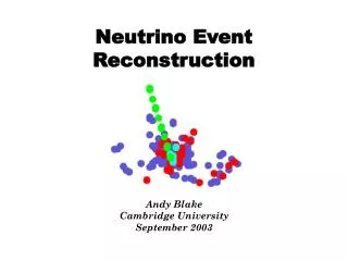
17. MiniBooNEParticleID ParticleID basically based on event topology e Real Data Event Display μ πo

18. MiniBooNEParticleID- space-time information What we know is actually the space and time distribution of charge An Event = {(xk, yk, zk), tk, Qk} k = 1, 2, …, NTankHits How to extract event topology from a set of PMT hits information The event topology is characterized by charge/hits fraction in space/time bins {(xk, yk, zk), tk, Qk} rk dtk = tk – rk/cn- t (ux, uy, uz) θ θc (x, y, z, t) s Point-like model

19. MiniBooNEParticleID– Construct input variables How to construct the ParticleID variables • Binning cosθin relative to event direction • - record hits/PMT number, measured/predicted charge, time/charge likelihood in each cosθ bin • Binning corrected time • - record hits number, measured/predicted charge, time/charge likelihood in each corrected time bin • Binning ring sharpness • - record hits/PMT number, measured/predicted charge, time/charge likelihood in each ring sharpness bin • Take physically meaningful ratio in certain bin • and combination of different bins • Dimensionless quantity is preferred

20. MiniBooNEParticleID– Other input variables Other ParticleID variables • Reconstruced physical observables: - e.g.πo mass, energy, track length and Cerenkov/scintillation light flux, production angle, etc. • Reconstructed geometrical quantities: - e.g. radius r, u· r, and distance along track to wall, etc. • Difference of likelihood between different hypotheses fitting: - electron/muon/pi0 fitting These variables are very powerful !

21. MiniBooNEParticleID– Use how many inputs How many variables do we need? At most, the number of variables we have {(xh, yh, zh), th, Qh} × NTank PMTs = 5 × NTank PMTs But they are highly correlated ! In ideal case, we can focus on the track instead of PMT hits. The least number of variables needed to describe one track is ~ 10 • Radius r - from tank center to MGEP • Angle α- between track and radial direction • Energy E • Light emision in unit length • - parametrized by some parameters (ux, uy, uz) r (x, y, z, t) α For πo events, twice as many variables needed.

22. MiniBooNEParticleID– How to select variables How to select ParticleID variables: reliability & efficiency ParticleID algorithm training and test have to rely on Monte Carlo 1. Does the variable distribution Data/MC agree ? Check with open box, cosmic ray calibration and NuMI data/MC 2. Does the correlation between variables Data/MC agree? The events number in each node of the trees can test correlation between variables, and can be used to look at data/MC comparison naturally. Energy/geometry variable dependence. These two requirements ensure output Data/MC agree and so the reliability of ParticleID 3. Is the variable/combination powerful in separation Too many inputs may degrade the ParticleID performance

23. MiniBooNEParticleID– Data/MC comparison The input data/MC comparison

24. MiniBooNEParticleID- Data/MC comparison The input data/MC comparison

25. MiniBooNEParticleID- Algorithm Choose which algorithm SC=Simple Cuts ANN=Artifical Neural Network BDT=Boosted decision tree Boosting is preferred in MiniBooNE to get better sensitivity but Simple Cuts method and ANN can provide cross check. Reasonably more input variables may result in higher performance, but less input variables may be more reliable.

26. MiniBooNEParticleIDBoosting Boosting – boosted decision tree A. Generate tree • Boosting: how to split node • – choose variable and cut Define GiniIndex = P (1 - P) ∑w(S+B) P =∑wS/∑w(S+B), w is event weight. For a pure background or signal node GiniIndex = 0 Start here For a given node, determine which variable and cut value maximizes variable = i Cut = ci G = GiniIndexFather – ( GiniIndexLeftSon + GiniIndexRightSon ) variable(i)<ci variable(i)>=ci 2. Boosting: how to generate tree – choose node to split Variable = k Cut = ck Among the existing leaves, find the one which gives the biggest G and split it. Repeat this process to generate a tree of the chosen size. variable(k)<ck variable(k)>=ck

27. MiniBooNEParticleID – Boosted decision trees B. Boost tree 3. Boosting: how to boost tree - Choose algorithm to change event weight Take ALL the events in a leaf as signal events if the polarity of that leaf is positive. Otherwise, take all the events as background events. Mark down those events which are misidentified. Reduce the weight of those correctly identified events while increase the weight of those misidentified evens. Then, generate the next tree. Define polarity of a node: polarity = + 1 if signal is more than background polarity = - 1 if background is more than signal C. Output 4. Boosting: how to calculate output value - Sum over (polarity × tree weight) in all trees See B. Roe et al. NIM A543 (2005) 577 and references therein for detail

28. MiniBooNEParticleID Simple Cuts and Boosted Decision Tree Simple Cuts Generalization Decision Tree Improvement All events Boosted Decision Tree variable = i Cut = c1 Var1<c1 || (var1>=c1 && var2<c2) Var1<c1 Var1>=c1 Simple Cutscan be taken as One Tree, Few Variables, Few Nodes variable = 2 Cut = c2 Var2<c2 Var2>=c2

29. MiniBooNEParticleID- conclusion on algorithm Some conclusions based on our past experience Boosting is better than Artificial Neural Network Boosting performance is higher in many variable (>20) case and relatively insensitive to detector MC in comparison to ANN Cascade Boosting is better than non-Cascade Boosting Cascade Boosting – build first boosting used as cut to select training events for second boosting, use second boosting Cascade Boosting training can improve 25~30% or even more relative to non-Cascade training, especially in low background contamination region Combine individual separation outputs can improve further By about 10~20%

30. MiniBooNEParticleID-Cascade Boosting Combine individual outputs 2nd boosting – cascade P r e l i m i n a r y 1st boosting - cascade

31. MiniBooNEParticleID– Output data/MC comparison The output data/MC comparison

32. MiniBooNEParticleID– Output data/MC comparison The output data/MC comparison

33. MiniBooNE ParticleID– How to play Event counting Optimize PID cuts to maximize Energy or/and ParticleID spectrum fitting After some precuts, do Energy spectrum fit PID output distribution fit Energy and PID two dimensional fit to get oscillation sensitivity

34. MiniBooNEEvent Reconstruction and Particle Identification Conclusion MiniBooNE Event Reconstruction provides Position resolution ~ 23cm Direction resolution ~ 6o Energy resolution ~ 14% Pi0 mass resolution ~ 23 MeV/c2 Based on the reconstruction information, with • Boosted decision trees • Cascade training • Combining specialist algorithms a much better ParticleID than BooNE proposal required ~ 67% electron efficiency 1% Pi0 contamination < 0.1% muon contamination has been achieved!