Understanding Transport Layer Congestion Control: A Deep Dive
Learn about congestion control principles, causes, and costs in the context of the transport layer. Explore scenarios, approaches, and TCP congestion control mechanisms in computer networking.


Understanding Transport Layer Congestion Control: A Deep Dive
E N D
Presentation Transcript
Chapter 3Transport Layer Computer Networking: A Top Down Approach 5th edition. Jim Kurose, Keith RossAddison-Wesley, April 2009. Transport Layer
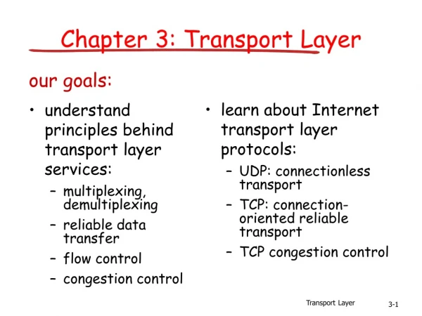
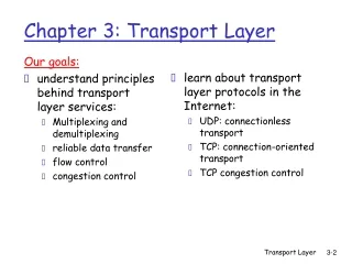
Our goals: understand principles behind transport layer services: multiplexing/demultiplexing reliable data transfer flow control congestion control learn about transport layer protocols in the Internet: UDP: connectionless transport TCP: connection-oriented transport TCP congestion control Chapter 3: Transport Layer Transport Layer
3.1 Transport-layer services 3.2 Multiplexing and demultiplexing 3.3 Connectionless transport: UDP 3.4 Principles of reliable data transfer 3.5 Connection-oriented transport: TCP segment structure reliable data transfer flow control connection management 3.6Principles of congestion control 3.7 TCP congestion control Chapter 3 outline Transport Layer
Congestion: informally: “too many sources sending too much data too fast for network to handle” different from flow control! manifestations: lost packets (buffer overflow at routers) long delays (queueing in router buffers) a top-10 problem! Principles of Congestion Control Transport Layer
two senders, two receivers one router, infinite buffers no retransmission large delays when congested maximum achievable throughput lout : per-connection throughput lin : original data rate unlimited shared output link buffers Host A Host B Causes/costs of congestion: scenario 1 C is outgoing link rate. Transport Layer
one router, finite buffers sender retransmission of lost packet Causes/costs of congestion: scenario 2 Host A lout lin : original data l'in : original data, plus retransmitted data Host B finite shared output link buffers l'in is the offered load. l'in > lin Transport Layer
always: (goodput) “perfect” retransmission only when loss: retransmission of delayed (not lost) packet makes larger (than perfect case) for same l l l > = l l l R/2 in in in R/2 R/2 out out out R/3 lout lout lout R/4 R/2 R/2 R/2 lin lin lin Causes/costs of congestion: scenario 2 Retrans. Due to Loss No Loss Retrans. Due to Loss And Premature Timeout “costs” of congestion: • more work (retrans) for given “goodput” • unneeded retransmissions: link carries multiple copies of pkt Transport Layer
four senders multihop paths timeout/retransmit l l in in Host A Host B Causes/costs of congestion: scenario 3 Q:what happens as and increase ? lout lin : original data l'in : original data, plus retransmitted data finite shared output link buffers Transport Layer
Host A Host B Causes/costs of congestion: scenario 3 lout Another “cost” of congestion: • when packet dropped, any “upstream transmission capacity used for that packet was wasted! Transport Layer
End-end congestion control: no explicit feedback from network congestion inferred from end-system observed loss, delay approach taken by TCP Network-assisted congestion control: routers provide feedback to end systems single bit indicating congestion (SNA, DECbit, TCP/IP ECN, ATM) explicit rate sender should send at Approaches towards congestion control Two broad approaches towards congestion control: Transport Layer
ABR: available bit rate: “elastic service” if sender’s path “underloaded”: sender should use available bandwidth if sender’s path congested: sender throttled to minimum guaranteed rate RM (resource management) cells: sent by sender, interspersed with data cells bits in RM cell set by switches (“network-assisted”) NI bit: no increase in rate (mild congestion) CI bit: congestion indication RM cells returned to sender by receiver, with bits intact Case study: ATM ABR congestion control Transport Layer
two-byte ER (explicit rate) field in RM cell congested switch may lower ER value in cell sender’ send rate thus maximum supportable rate on path EFCI bit in data cells: set to 1 in congested switch if data cell immediately preceding RM cell has EFCI set, destination sets CI bit in returned RM cell Case study: ATM ABR congestion control Transport Layer
3.1 Transport-layer services 3.2 Multiplexing and demultiplexing 3.3 Connectionless transport: UDP 3.4 Principles of reliable data transfer 3.5 Connection-oriented transport: TCP segment structure reliable data transfer flow control connection management 3.6 Principles of congestion control 3.7 TCP congestion control Chapter 3 outline Transport Layer
TCP congestion control: additive increase, multiplicative decrease • Approach: increase transmission rate (window size), probing for usable bandwidth, until loss occurs • additive increase: increase cwnd by 1 MSS every RTT until loss detected • multiplicative decrease: cut cwnd in half after loss Saw tooth behavior: probing for bandwidth congestion window size time Transport Layer
sender limits transmission: LastByteSent-LastByteAcked cwnd Roughly, cwnd is dynamic, function of perceived network congestion How does sender perceive congestion? loss event = timeout or 3 duplicate acks TCP sender reduces rate (cwnd) after loss event three mechanisms: AIMD slow start conservative after timeout events cwnd rate = Bytes/sec RTT TCP Congestion Control: details Transport Layer
When connection begins, cwnd = 1 MSS Example: MSS = 500 bytes & RTT = 200 msec initial rate = 20 kbps available bandwidth may be >> MSS/RTT desirable to quickly ramp up to respectable rate TCP Slow Start • When connection begins, increase rate exponentially fast until first loss event Transport Layer
When connection begins, increase rate exponentially until first loss event: double cwnd every RTT done by incrementing cwnd for every ACK received Summary: initial rate is slow but ramps up exponentially fast time TCP Slow Start (more) Host A Host B one segment RTT two segments four segments Transport Layer
After 3 dup ACKs: cwnd is cut in half window then grows linearly But after timeout event: cwnd instead set to 1 MSS; window then grows exponentially to a threshold (ssthresh), then grows linearly Refinement: inferring loss Philosophy: • 3 dup ACKs indicates network capable of delivering some segments • timeout indicates a “more alarming” congestion scenario Transport Layer
Q: When should the exponential increase switch to linear? A: When cwnd gets to 1/2 of its value before timeout. Implementation: Variable Threshold (ssthresh) At loss event, ssthresh is set to 1/2 of cwnd just before loss event Refinement Transport Layer
Summary: TCP Congestion Control • When cwnd is below ssthresh, sender in slow-start phase, window grows exponentially. • When cwnd is above ssthresh, sender is in congestion-avoidance phase, window grows linearly. • When a triple duplicate ACK occurs, ssthresh set to cwnd/2 and cwnd set to ssthresh. • When timeout occurs, ssthresh set to cwnd/2 and cwnd is set to 1 MSS. Transport Layer
TCP sender congestion control Transport Layer
TCP throughput • What’s the average throughput of TCP as a function of window size and RTT? • Ignore slow start • Let W be the window size when loss occurs. • When window is W, throughput is W/RTT • Just after loss, window drops to W/2, throughput to W/2RTT. • Average throughout: .75 W/RTT Transport Layer
TCP Futures: TCP over “long, fat pipes” • Example: 1500 byte segments, 100ms RTT, want 10 Gbps throughput • Requires window size W = 83,333 in-flight segments • Throughput in terms of loss rate: • ➜ L = 2·10-10 Wow • New versions of TCP for high-speed Transport Layer
Fairness goal: if K TCP sessions share same bottleneck link of bandwidth R, each should have average rate of R/K TCP connection 1 bottleneck router capacity R TCP connection 2 TCP Fairness Transport Layer
Two competing sessions (AIMD): Additive increase gives slope of 1, as throughout increases multiplicative decrease decreases throughput proportionally Why is TCP fair? equal bandwidth share R loss: decrease window by factor of 2 congestion avoidance: additive increase Connection 2 throughput loss: decrease window by factor of 2 congestion avoidance: additive increase Connection 1 throughput R Transport Layer
Fairness and UDP Multimedia apps often do not use TCP do not want rate throttled by congestion control Instead use UDP: pump audio/video at constant rate, tolerate packet loss Research area: TCP friendly Fairness and parallel TCP connections nothing prevents app from opening parallel connections between 2 hosts. Web browsers do this Example: link of rate R supporting 9 connections; new app asks for 1 TCP, gets rate R/10 new app asks for 11 TCPs, gets R/2 ! Fairness (more) Transport Layer
principles behind transport layer services: multiplexing, demultiplexing reliable data transfer flow control congestion control instantiation and implementation in the Internet UDP TCP Next: leaving the network “edge” (application, transport layers) into the network “core” Chapter 3: Summary Transport Layer