Download
1 / 47
470 likes | 709 Vues
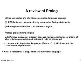
A review of Prolog. • will be our choice of a shell implementation language because (i) KBS facts and rules are directly encoded as Prolog statements (ii) Prolog has built within it an inference engine • Prolog: pro gramming in log ic

E N D
A review of Prolog • will be our choice of a shell implementation language because (i) KBS facts and rules are directly encoded as Prolog statements (ii) Prolog has built within it an inference engine • Prolog: programming in logic • a declarative language: program code are human-oriented descriptions of what is being computed, and not how it is to be computed - compare with imperative languages (Pascal, C,...) which encode the computational procedure • Note: a competitor is Lisp, which is a functional language
Logic • 1st order predicate logic: a mathematical theory which models the world with sentences denoting truth eg. Either it rains or it does not rain. Every number different than 0 is the successor of another number. If Jack is the parent of Fred, then Jack is the father of Fred, or Jack is the mother of Fred. If Jack is the parent of Fred, and Jack is male, then Jack is the father of Fred. There exists someone who is a parent of Fred. • predicate logic is concerned with: - formally representing facts with a formal grammar ('Predicate logic") - determining ways of deducing logical truths from these sentences "deduction"
Logic Rules for connectives: ~W is true if and only if W is false W1 & W2 is true if and only if W1 is true and W2 is true W1 or W2 is true if and only if either W1 is true or W2 is true W1 if W2 is false if and only if W1 is false and W2 is true W1 iff W2 is true if and only if either both W1 and W2 are true or both W1 and W2 are false Rules for Quantifiers: ( ∀ X ) W is true if and only if W is true for every substitution of a domain object for X within W ( ∃ X ) W is true if and only if W is true for at least one substitution of a domain object for X
Logic • If a sentence contains quantifiers and variables, in order to determine the truth of the sentence, you need to define a domain from which objects will be selected. eg. (∀ X ∃ Y) likes(X, Y) --> need to determine what X and Y are representing: ie. people? Food? integers?... • whether the sentence is really true depends on the model you define • the pairs of objects in which "likes(X,Y)" is defined by a relation • a relation is a set of tuples that are deemed to be true eg. if domain is { john, joe, mary, jane } then the relation for likes in our model might be: likes= { (john, joe), (mary, john), (jane, jane)} So likes(X,Y) is true for likes(john, joe), likes(mary, john), likes(jane, jane)
Logic • if a given sentence is true for at least one model, then it is satisfiable otherwise it is unsatisfiable eg. (∀ X ∃ Y) likes (X, Y) iff ~likes(X,Y) is unsatisfiable • some sentences are always true: tautologies eg. (∀ X) p(X) & p(X) iff p(X) • existential quantification makes logic complex: there is no automatic means for finding the object which satisfy an existential equation - you can have an infinite set of objects to consider, so it would require exhaustively searching the set
Logical deduction • S1 ⊨ S2 - S2 is a logical consequence of sentence(s) S1 eg. (∀ X) likes(chris, X) ⊨ likes(chris, mum) • S1 ⊢ S2 - S3 is derivable from S1 eg. (∀ X,Y) likes(X,Y) or true ⊢ true • the useful part of logic is that it is possible to apply syntactic transformations of sentences which preserve their truth in the model being represented by the sentence denoted: ∀ P, Q P ⊨ Q iff P ⊢ Q • there are many procedures for deriving new sentences, and hence new statements of truth • automatic theorem proving is concerned with proving a sentence is true, by applying syntactic transformations to it
Logical deduction • logic programming technique: (a) convert statements of logic into Horn clauses (exists an algorithm to do that) (∀ X's) p(X's) if q1(X's) & ... & qn(X's) (∀ X's) p(X's) note: can have terms as arguments in predicate tuples (WFF's) • logic programming languages use the following deduction rule (called modus ponens): { ~A, (A if B) } ⊢ ~B { ~A, A } ⊢ false • this rule preserves soundness ie. truth is maintained.
Logic Programming • logic programming languages use the following notation: (∀ X's) p(X's) if q1(X's) & ... & qn(X's) (∀ X's) p(X's) p(X's) :- q1(X's), ... , qn(X's). <-- called a "rule" p(X's). <-- called a "fact" • This restricted notation is just as computationally powerful as full predicate logic
Syntax Constants: name specific objects i) atoms: constants or symbolic terms - constants begin with lower-case letter eg. bob, x25, aDog, - symbols are such things as =, +, ... (might be predefined in implementation, eg. :- ) ii) integers: 0, 25, -5 Variables: are generic place-holders of constants - begin with upper-case letter - eg. Answer, L, My_List, A3 - anonymous variable: the underscore _ , used when you don't need to use that variable anywhere else
Syntax (cont) Structures : basic data structure term constant(arg 1, arg 2, ..., arg k) k 1 - eg. bob(25), age(old), age(X), tree(left(X), right(L)), *(4), ... illegal: B(bob) - there are useful buiiltin structures, for example... lists [] - empty list , short for '.'() [H|T] - list with first element H and tail list T, '.'(H,T) eg. [a,b,c], [25], [ _ ], [ t(a,b), t(X,Y), Z] • Term: a constant, variable, or structure
Prolog Statements • Three basic kinds of statements 1. facts: parent(john, P). bank_account(36569483, smith, john, 25.66). finished. 2. rules: parent(X,Y) :- father(X,Y). grandparent(X,Y) :- parent(X,Z), parent(Z,Y). op_sys :- input(Job), run(Job,Res), cleanup(Res). 3. query: :- parent(jane,W). :- parent(X,Y), parent(Y,Z).
Logic Programming fact or assertion • real example: append([ ], X, X). append([A|X], Y, [A|Z] ) :- append(X, Y, Z). rule head body • each fact or rule is called a clause • all the clauses with the same head name and # of arguments is a predicate (akin to a procedure)
Program structure • predicate: all the clauses having the same identifier and number of arguments is - akin to a procedure • eg. parent(X,Y) :- father(X,Y). parent(X,Y) :- mother(X,Y). parent(adam). father(john, tim). father(john, jane). mother(jane, jill). grandparent(X,Y) :- parent(X,Z), parent(Z,Y). grandparent(adam, _). grandparent(eve, _). human_being(_). mother(john, tim).
Prog. structure (cont) Good programming practices: - group all clauses of a predicate together in program file - be careful using same predicate identifier with different # args - never put more than one clause per line. - For large rules, put one goal per line also. eg. grandfather(X,Y) :- male(X), parent(X,Z), parent(Z,Y).
Unification • Computing solutions: a powerful feature of logic programming systems is their ability to substitute values into the variables found in clauses - this lets the deduction compute values to a query • unification: pattern matching technique in which two atoms are matched together, and produces the most general substitution of variables that makes the 2 atoms identical • method: (i) two variables always unify: X = Y (ii) a variable always unifies with a non-variable term that does not contain that variable: X = s(Y, d(Q)) (iii) two non-var terms unify if their arguments unify : s(W, Y) = s(X, c) (because W = X and Y = c) • when a variable unifies with a term, we say it is bound to that term this binding is a data binding that holds forever ( until backtracking )
Unification examples • c = c --> result: 'true' • X = Y (where X, Y are uninstantiated) --> result: X <- Y (they are matched together) • X = d --> result: X <- d • s(X) = s(Y,c) --> fail • t(c) = t(Z) --> result: Z <- x • apples = oranges --> fail • apples = Apples --> result: Apples <- apples • a(b,C,d(e,F,g(h(i,J)))) = a(B,c,d(E,f,g(H))) --> result: B <- b, C <- c, E <- e, F <- f, H <- h(i,J)
Unification (cont) • Note: unification can produce infinite terms, or even never terminate, under some conditions - this happens when the same variable occurs in both expressions eg. Y = father(Y) --> result: Y <- father(father(father(..... ))) – this usually only happens by accident in buggy programs
Substitutions • the computed result from unification procedure • Also called bindings or computed answer substitutions • have form: Ω = { X1 <- t1,... Xk <- tk } ( k 0 ) where Xi's are variables and ti's are terms (constants, structures, variables) • each variable Xi is distinct To apply a substitution to a term: • simultaneously substitute all terms ti for the Xi in the term eg. let term W = p(U, g(V), Y) Ω = {U <- a, V <- Y, Y <- c} then W Ω = p(a, g(c), c) Note: it can simplify things to apply Y <- c for V in
Unification algorithm Input: two terms T1 and T2 to be unified Output: the answer substitution set Ω, or FAIL Initialize: Ω := empty Algorithm: 1. If T1 (or T2) is a variable: (a) If variable T1 (or T2) occurs in expression T2 (or T1) then FAIL (b) else add T1 <- T2 (or T2 <- T1) to Ω, and reset T1 everywhere else 2. if either expression is a constant, and the other expression is a different constant or structured term, then FAIL 3. If both expressions are structured terms: (a) if they have different identifiers OR different # arguments then FAIL (b) else apply unification recursively to their arguments, unifying then by their corresponding ordered positions
More examples 1) s(X, t(T ,X), Z) = s(a, t(b, c), W) 2) [ a, f(B), C, d, e, f ] = [ First, Second, Third | Rest ]
Resolution • basic computation technique in logic programming • given a query :- G1, G2,...,Gk and a set of program clauses of form H :- B1, B2,..., Bj. (j≥0) 1. select a goal Gi (1 ≤ i ≤ k) in the query 2. find a clause Hn whose head unifies Gi resulting in a set of unification bindings Ω (might be empty) 3. replace Gi by the body of Hn, and apply to new query ie. G1,...,G(i-1),Gi, G(i+1),...,Gk. Hn :- B1n,B2n,...,Bmn. (G1,...,G(i-1), B1n,B2n,...,Bmn, G(i+1),...,Gk.) 4. Repeat until an empty query is obtained; all the Ω 's collected will give the solution to the computation
Resolution trees • Note that there are many ways to select a goal in the query to process next, and many ways to select a candidate clause in the program • The computation can be represented by a tree: :- Q1 Hk Hi Hj :- Q2 :- Q3 :- Q2 Hm Hr Hl :- Q5 :- Q4 Hn Hq Hp Ho (fail) (success)
Logic Programming • example deduction using resolution: Program P: C1: A :- B. Query: ?- A. (notation for queries) C2: B :- C. C3: B :- D, F. C4: D :- E. C5: D . C6: E. C7: F. (1) ?- A. apply C1: ?- B. apply C3: ?- D, F. apply C7: ?- D. apply C4: ?- E. apply C6: ?- nil. --> thus ~A is false, or A is true. (2) ?- A. apply C1: ?- B. apply C3: ?- D, F. apply C5: ?- F. apply C7: ?- nil --> ditto.
Prolog's Control • from previous examples, note that deduction proof 2 is shorter. Issues: (1) which clause to apply? (2) which goal in query to reduce? • Unfortunately, there is no automatic means of deciding this. • logic programming interpreters will use some sort of arbitary scheme • Prolog's Standard depth-first left-to-right control: a) control rule: always pick left-most goal to reduce b) search rule: always pick first clause that matches c) when there is no clause to apply, then go back to where you had a choice of clauses to choose from, and choose the next one --> "backtracking" • (c) above lets the interpreter find multiple solutions to a query • advantage: It's easy to learn, and efficient to implement • disadvantage: it is unfair, and tree searches can be nonterminating (contrast with breadth-first control)
Backtracking • refers to searching for multiple solutions • a by-product of searching more than one clausewhen computing a goal 1: plan_date(Guy, Gal, Food) :- likes(Guy, Food), likes(Gal, Food). 2: likes(tom, sushi). 3: likes(tom, pasta). 4: likes(tom, bbq). 5: likes(sue, pasta). 6: likes(sue, bbq). ?- plan_date(tom, sue, Food) 1 ?- likes(tom,Food), likes(sue, Food) 2 3 4 ?- likes(sue, sushi) ?- likes(sue, pasta) ?- likes(sue, bbq) 5 6 { Food <- bbq } {Food <- pasta }
Backtracking • Variables are unique within each clause. • when recursion occurs, rename variables in the clause so that they don't clash with those in the current goal eg. grandparent(A,B) :- parent(A,X), parent(X,B). parent(X,Y) :- father(X,Y). parent(X,Y) :- mother(X,Y). ?- grandparent(X, tom). ( grandparent(A,B) :- parent(A, X' ) , parent(X' , B). ) = { X <- A, B <- tom } ?- parent(A, X'), parent(X', tom).
Some possible program behaviors - no solutions: output --> "no" eg. ?- pet(cat). pet(dog). - a finite number of solutions eg. ?- pet(X). pet(cat). pet(dog). - an infinite number of solutions eg. ?- pet(Y). pet(dog). pet(X) :- pet(X). - non-termination, and eventually memory overflow eg. ?- pet(X). pet(Y) :- pet(Y). - computation error: bad use of builtin predicates
Real Prolog • Real prolog implementations add extra-logical features so that practical programming can be done. Some examples from Clocksin & Mellish are: (1) Input-Output: read\1, write \1 - read and write terms get\1, pur\1 - read and write characters nl - write a new line (2) Files see(X) - opens file X for input tell(X) - opens file X for output (3) Negation not G - succeeds if goal G fails, and fails if G succeeds (3) Equality X = Y - unifies X and Y, or fails if they don't unify X \= Y - opposite of X = Y, ie. not (X = Y) X == Y - like X=Y, except that all variables have to be the same too; == does not instantiate any variables
Real prolog 3. equality (cont) X \== Y - same as: not X == Y 4. integer relations: < > >= =< = \= eg. X < Y - succeeds if value in X < Y. Note that X and Y can't be uninstantiated 5. arithmetic: X is Expr - where Expr is an arithmetic expression using +, - , *, /, mod, ... - (i)Y op Z is evaluated,; (ii) if X is not set, it is set to expr's value, or (iii) if X has a value, then it is compared with expression value. - Note that arithmetic expressions must use instantiated variables, else ERROR. 6. program database manipulation asserta(G), assertz(G) - adds clause G to the program database retract(G) - matches G with a clause, and removes it if found retractall(H) - retracts all clauses whose heads match with H
Real Prolog 7. control repeat - always succeeds fail - always fails eg. loop :- repeat, write('hi!'), nl, fail. 7. structure manipulation S =.. List - Structure S is decomposed into List, or List is converted to S eg. A =.. [stock, macintosh, 128k] : A <- stock(macintosh, 128k) stock(pc2, 640k, mouse) =.. L : L <- [stock, pc2, 640k, mouse] eg. Testing the name of an atom checkname(Struct, Ident) :- Struct =.. [Ident| _ ]. ?- checkname(stock(pc2,64K,...), A). A = stock.
Real Prolog 8. Variable inspection var(X) - succeeds if X is an uninstantated variable nonvar(X) - suceeds if X is not instantiated integer(X) - succeeds if X is an integer 9. program inspection clause(H,B) - matches head H and body B with a clause in database (facts have 'true' set for body) 10. atom inspection name(A,L) - breaks name A into a list L of integer ascii values eg. name(apple,L) : L <- [97, 112, 112, 108, 100] And Much More
The Cut: ! • Used to permit more control over search. It deletes or 'cuts' parts of the computation tree. (1) p(X) :- q(X,Y). (2) p(X) :- r(X,Y), !, s(Y). (3) p(X) :- t(Y). ?- p(X). i) All the solutions from (1) are used. ii) If r(X,Y) succeeds, then ! is activated: - during backtracking, if s(Y) fails, then the whole clause fails - also, solutions from (3) will be ignored iii) if r(X,Y) fails, then (2) fails, and computation proceeds to (3) Note that s(Y) can still return multiple solutions
Cut (cont) • Common use of cuts: p(X) :- G1, ..., Gk, !. : this means that, if clause succeeds, it will only return 1 solution eg. make member only return 1 solution member(X, [X| _ ]) :- !. member(X, [_ |Y]) :- member(X,Y). • possible to create cleaner control constructions with the cut eg. once(P) :- call(P), !. or once(P) :- P, !. eg. if_then_else(P, Q, R) :- P, !, Q. if_then_else(P, Q, R) :- R. ( could be : if_then_else(P, Q, R) :- P, Q. if_then_else(P, Q, R) :- (not P), R. except that test P might be expensive. )
Meta-interpreters • meta-interpreter: interpreter for a language written in the language itself • Prolog is ideally suited for this: solve(true). solve(not(A)) :- not solve(A). solve((A,B)) :- solve(A), solve(B). solve(A) :- clause(A,B), solve(B). goals in Prolog are stored as: A, (B, (C, D)) ie. "," is right-associative builtin predicate which gets a clause which unifies with head A, and has body B
Defining operators • Prolog lets you define your own operators (or override builtin ones) • useful for writing customized programs, especially meta-interpreters eg. ?- op(300, yfx, ^). executed goal! right-associative infix: 2^3^4 --> 2^(3^4) relative precedence • to set precedence, you need the precedence settings of the system your using • see Clocksin & Mellish for explanation of op definitions
Disjunction, if-then-else • disjunction (logical OR): parent(Parent, Child) :- mother(Parent, Child) ; father(Parent, Child). - can also do: p(X, Y) :- ( a(X, Z), b(Z, Y)) ; c(Y). - whenever you see a ";", you can convert the clause into multiple clauses • If - then : parent(X, Y) :- person(X) -> mother(X, Y). - behaves almost like parent(X,Y) :- person(X), mother(X, Y). except that person only returns one solution (no backtracking when mother fails) • If - then - else: parent(X, Y) :- male(X) -> father(X, Y) ; mother(X, Y). - if male(X) true, then father executed, else mother executed
If-then-else • if-then-else can often be used instead of cuts • implemented as: parent(X, Y) :- male(X), !, father(X, Y). parent(X, Y) :- mother(X, Y). • trick: once(P) :- call(P), !. <-- this saves putting cuts in lots of clauses eg. once(member(apple, L)) <- don't need a "member" that has a cut in it
Debugging Prolog • interpreter's trace facility is very useful • standard debugging features: spy - set a breakpoint on a procedure trace - manually control execution skip - call a goal, and return control when goal finished creep - trace into the goal call redo - call goal again fail - force goal to fail • Beware! If you change the database (assert, retract), be sure to clean it up if necessary. Otherwise, you'll get side effects (doubly asserted clauses, etc)
Example Prolog programs • Lists • graph searching • graph searching with cycle checking • bubble sort • sorted binary tree
Example 1: appending lists append( [ ], L, L). append( [X | R] S, [X | T]) :- append(R, S, T). ?- append([ a, b, c], [1, 2, 3], L). L = [a, b, c, 1, 2, 3] . ?- append( Y, [1, 2, 3], [a, b, c, 1, 2, 3]). Y = [a, b, c] ?- append(X, Y, [1,2,3]). X=[ ], Y = [1, 2, 3] ; X=[1], Y = [2, 3] ; X=[1,2], Y = [3] ; X = [1,2,3], Y = [ ]; no ?- append([_|_], [Y|_], [1, 2, 3]). % a way to use append like ‘member’! Y = 1; Y = 2; Y = 3; no
Example: sorted binary trees nil : empty branch/tree tree(Left_branch, Key, Right_branch) : tree node with data • hence tree(tree(nil,2,nil), 4, tree(tree(nil,5,nil), 6, nil)) represents: 4 2 6 5
Binary tree (cont) add_bintree(Key, nil, tree(nil, Key, nil). add_bintree(Key, tree(L, Key, R), tree(L, Key, R)). add_bintree(Key, tree(L, K, R), tree(L2, K,R)) :- Key < K, add_bintree(Key, L, L2). add_bintree(Key, tree(L, K, R), tree(L, K, R2) :- Key > K, add_bintree(Key, R, R2).
Example: graph search i a 5. Representing directed graphs as program clauses edge(d, c). edge(f, e). edge(h, l). edge(b, c). edge(f, i). edge(l, k). edge(b, f). edge(i, j). edge(g, f). edge(a, b). edge(j, k). edge(g, h). edge(e, f). edge(k, g). j f g k b h e l c d
Graphs • Graphs (cont) • Can then search for connections within the graph: path(A, B) :- edge(A,B). path(A,B) :- edge(A,C), path(C,B). note similarity with ‘ancestor’: ancestor(A,B) :- parent(A,B). ancestor(A,B) :- parent(A,C), ancestor(C,B). • However, unlike family relationships, graphs can have loops • using Prolog’s backtracking, it can easily get sidetracked into a loop • eg. ?- path(j,a) will go thru: j - k - g - f - i - j - etc
Graphs • Graphs: another approach: use a list structure [v(Node1, Nodelist1), v(Node2, Nodelist2), ...] then graph([ v(a, [b, f]), v(b, [c,f]), v(d, [f]), v(f, [e,i]), v(g, [f,h]), v(i, [j]), v(j, [k]), v(k, [g]), v(l, [k]), v(h, [l]) ] ). • Can write a ‘path’ routine which keeps track of places it has already been to; if it has been to a place already, then don’t go there again! (can also do this with the other representation)
Graphs path(Start, Finish) :- graph(G), smart_path(Start, Finish, G, [ ]). smart_path(A, B, G, _) :- member(v(A,L), G), member(B, L). smart_path(A, B, G, Previous) :- member(v(A,L), G), member(C, G), not member(C, Previous), smart_path(C, B, G, [A | Previous]).
Bubble Sort bubble(L, S) :- append(X, {A,B|Y], L), B < A, !, append(X, [B, A | Y], M), bubble(M, S). bubble(L, L).