Nanoscale Modeling & Computational Infrastructure
Explore atomistic simulations, molecular dynamics, & multiscale modeling paradigms for predicting device performance & reliability in microsystems. Conduct PRISM experiments & develop constitutive relationships for numerical simulations.

Nanoscale Modeling & Computational Infrastructure
E N D
Presentation Transcript
Nanoscale Modeling and Computational Infrastructure___________________________Ananth GramaProfessor of Computer Science, Associate Director, PRISM Center for Prediction of Reliability, Integrity, and Survivability of MicrosystemsPurdue Universityayg@cs.purdue.edu, http://www.cs.purdue.edu/homes/ayg
PRISM Modeling Paradigms • Key Challenge: Scaling from femtosecond bond activity to predictions of billion-cycle performance • DFT for atomistic resolution • Reactive Molecular Dynamics for surface chemistry • Molecular dynamics for materials properties • Material Point Methods for bulk materials • Finite Volume Methods for fluid damping
PRISM Multi-physics Integration Predictions Trapped charges in dielectric Electronic processes Validation Experiments: Microstructure evolution, device performance & reliability PRISM Device simulation MPM & FVM Elastic, plastic deformation, failure Micromechanics Defect nucleation & mobility in dielectric Fluid damping Fluid dynamics Temperature and species Dislocation and vacancy nucleation & mobility in metal Atomistics Thermal and mass transport Fluid-solid interactions Thermal & electrical conductivity Input Experiments: Surface roughness, composition, defect densities, grain size and texture
Atomistic Simulations in PRISM Develop first principles-based constitutive relationships and provide atomic level insight for coarse grain models • Identify and quantify the molecular level mechanisms that govern performance, reliability and failure of PRISM device using: • Ab initio simulations • Large-scale MD simulations
Atomistic Modeling of Contact Physics Interatomic potentials Implicit description of electrons How: Reactive/Classical MD with ab initio-based potentials Size: 200 M to 1.5 B atoms Time scales: nanoseconds Predictions: Role of initial microstructure & surface roughness, moisture and impact velocity on: Force-separation relationships (history dependent) Generation of defects in metal & roughness evolution Mechanical response: Generation of defects in dielectric (dielectric charging) Thermal role of electrons in metals Current crowding and Joule Heating Electronic properties: Surface chemical reactions Chemistry: Main Challenges
Atomistic modeling of Contact Physics Smaller scale (0.5 – 2 M atom) and longer time (100 ns) simulations to uncover specific physics: • Mobility of dislocations in metal, • Interactions with other defects • Link to phase fields • Surface chemical reactions • Reactive MD using ReaxFF • Defects in semiconductor • Mobility and recombination • Role of electric charging • Fluid-solid interaction: • Interaction of single gas molecule with surface (accommodation coefficients) for rarefied gas regime
Obtaining Surface Separation-Force Relationships • Contact closing and opening simulation • 200 M to 1.5 billion atoms – nanoseconds • (1 billion atom for 1 nanosecond ~ 1 day on a petascale computer) • Characterize effect of: • Impact velocities • Moisture • Applied force and stress • Surface roughness • Peak to peak distance and RMS • Presence of a grain boundary
Upscaling MD to: Fluid Dynamics pi Given a distribution of incident momenta characterize the distribution of reflected momenta (accomodation coefficients) Fluid FVM models use accommodation coefficients from MD and predict incident distribution Role of temperature and surface moisture on accommodation coefficients
Upscaling MD to Electronic Processes • Defect formation energies • Equilibrium concentration • Formation rates if temperature increases • Impact generated defects • Characterize their energy and mobility as a function of temperature • Predict the distribution non-equilibrium defects • Characterize energy level of defects
Upscaling MD to Micromechanics • Elastic constants • Vacancy formation energy and mobility • Bulk and grain boundaries • Dislocation core energies • Screw and edge • Dislocation nucleation energies • At grain boundaries, metal/oxide interface • Nucleation under non-equilibrium conditions (impact) • Dislocation mobility and cross slip • Interaction of dislocations with defects • Solute atoms and grain boundaries Upscaling MD to Thermals • Thermal conductivity of each component • Interfacial thermal resistivity • Role of closing force, moisture and temperature
Computational Challenges • Development of effective algorithms for constitutive modeling paradigms • Reactive MD, classical MD • Effective solvers for sparse linear systems • Coupling and information transfer (upscaling, fluid- structure interaction, etc.
Bond order for C-C bond Bond Order Interaction • Uncorrected bond order: where is for andbonds • The total uncorrected bond order is sum of three types of bonds • Bond order requires correction to account for the correct valency
Parallel Performance Reactive and non-reactive MD on 131K BG/L processors. Total execution time per MD step as a function of the number of atoms for 3 algorithms: QMMD, ReaxFF,conventional MD [Goddard, Vashistha, Grama]
Parallel Performance Total execution (circles) and communication (squares) times per MD time for the ReaxFF MD with scaled workloads—36,288 x p atom RDX systems (p = 1,..,1920).
f1 A1 x1 B1 f2 x2 C2 A2 f3 x3 B2 = C3 A3 f4 x4 B3 C4 A4 Next Generation Sparse Solvers: The SPIKE Algorithm Ax = f • Solve Dy = f • Solve Sx = y A = D S D = diag (A1, A2, A3, A4)
SPIKE: Excellent Predictable Performance! N k p Observed Model 5, 000, 000 35 128 2.78 2.64 5, 000, 000 25 128 1.55 1.49 5, 000, 000 15 128 0.70 0.66 5, 000, 000 35 256 1.49 1.33 5, 000, 000 25 256 0.79 0.75 5, 000, 000 15 256 0.35 0.33 5, 000, 000 35 512 0.67 0.67 5, 000, 000 25 512 0.38 0.38 5, 000, 000 15 512 0.20 0.17 5, 000, 000 35 1, 024 0.37 0.35 5, 000, 000 25 1, 024 0.21 0.20 5, 000, 000 15 1, 024 0.10 0.09 Benchmarks on TACC Ranger Sun Constellation Cluster.
Summary • Highly innovative algorithms and parallel formulations for supporting next generation of nanoscale modeling challenges