THE HEIGHT OF LIQUID METHOD FOR FREE SURFACE FLOWS

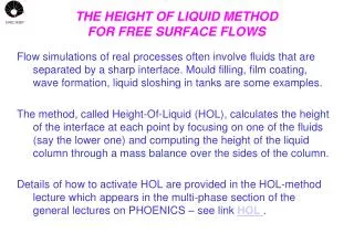
1. THE HEIGHT OF LIQUID METHOD FOR FREE SURFACE FLOWS Flow simulations of real processes often involve fluids that are separated by a sharp interface. Mould filling, film coating, wave formation, liquid sloshing in tanks are some examples. The method, called Height-Of-Liquid (HOL), calculates the height of the interface at each point by focusing on one of the fluids (say the lower one) and computing the height of the liquid column through a mass balance over the sides of the column. Details of how to activate HOL are provided in the HOL-method lecture which appears in the multi-phase section of the general lectures on PHOENICS – see link HOL .

2. APPLICABILITY AND RESTRICTIONS The only restriction is that the flow considered should exhibit no "overturning" of the interface. This means that there must exist one direction, designated the "up" direction, along which only ONE intersection of the interface exists. • The HOL method is applicable to: • Incompressible flows; • Steady and unsteady flows; • Two- or three-dimensional flows; • Cartesian, polar or curvilinear coordinates.

3. INTERFACE & OTHER DEFINITIONS • Interface – defines the boundary between two immiscible fluids (gas-liquid) or (liquid-liquid) • Representation of the numerical grid superposed to the interface. • The domain is composed by vertical slices, aligned with g, each one displaying a column of heavier liquid.

4. INTERFACE DISPLACEMENT ON A SLICE OF CELLS • The interface position is determined by a volumetric balance applied to vertical cell columns (incompressible & no overturning). • The volume imbalance at the cell where the interface lays will displace it upward or downward.

5. FRACTION OF LIQUID ‘VOF’ • VOF is the volumetric fraction of the cell occupied by the heavier fluid. • VOF =1 heavier fluid; VOF = 0 lighter fluid and 0<VOF<1 interface. • In a column of cells just one cell will have 0<VOF<1.

6. TIME STEP AND CELL DIMENSIONS • Tracking the interface requires a transient simulation. • The time step and the cell size must be balanced such that the interface stays at least one (usually five or more) time steps to leave one cell. • If the time step and the cells sizes are not balanced it may happen that in a single time step the interface may travel more than one cell while in the neighboring slices it doesn’t happen. • The balance of time step and cell size is defined case by case. • It is done by estimating the maximum velocity, choosing on cell size accordingly to the spatial resolution required and fixing a time step at least five times less than the ratio between the cell size and the maximum velocity.

7. WORKSHOP HOL #1 • GEOMETRY • DOMAIN SIZE (X,Y,Z) = (0.1, 0.5, 1) • GRID SIZE: AUTO • TRANSIENT: TIME = 25S & TIME STEPS = 50 • MODELS • VELOCITY: LAMINAR • FREE SURFACE MODEL: HOL; HEIGHT DIRECTION: +Z

8. WORKSHOP HOL #1 • PROPERTIES • LIGHT FLUID: AIR (0) • HEAVY FLUID: WATER (67) • DOMAIN INITIALLY FULLY: LIGHT FLUID • OBJECTS • INLET: SIZE (0.1, 0.1, 0) PLACE (0,0,0) W = +0.1M/S INLET DENSITY: HEAVY • OUTLET: SIZE (0.1, 0.5, 0) PLACE (0,0,1) • INITIALIZATION • V1 = 0; W1 = 0.1; VOF = 0

9. WORKSHOP HOL #1 • SOURCES • NUMERICS • NUMBER OF ITERACTIONS: 10 • RELAX: AUTO OFF • RELAX: FALSDT 1E-03 FOR V1, W1 • OUTPUTS FIELD DUMPING

10. WORKSHOP HOL #1 • Get the VOF instantaneous contour maps. • Where is the interface

11. INTERFACE LOCATION • The interface position is not known precisely, what is known is the fraction of volume in each cell. • Notice that the interface is where 0 < VOF < 1, see not-averaged contour plot. • One possibility is to admit that the free interface coincides with the points where VOF = 0.5.

12. SOLUTION REFINEMENT • Is the VOF, velocities and pressure fields fully converged • Set time steps to 150; change the dumping fields frequency to 12 and compare the solution with the previous run. • Answer if the liquid sloshing observed on the previous run still exists Also observe the velocity vector fields.

13. SLUMPING OF A LIQUID COLUMN BY HOL • Load library case P102 • Set the view to –X and up direction to +Z • Change the number of iterations to 100. • Inspect the blockages, and all other objects. • Run the case

14. END

15. INTERFACE & OTHER DEFINITIONS • Interface – defines the boundary between two immiscible fluids (gas-liquid) or (liquid-liquid) • Representation of the numerical grid superposed to the interface. • The domain is composed by vertical slices, aligned with g, each one displaying a column of heavier liquid. LIGHTER FLUID HEAVIER FLUID

16. INTERFACE DISPLACEMENT ON A SLICE OF CELLS • The interface position is determined by a volumetric balance applied to vertical cell columns (incompressible & no overturning). • The volume imbalance at the cell where the interface lays will displace it upward or downward. To conserve the volume the interface has to displaced upward

17. FRACTION OF LIQUID ‘VOF’ • VOF is the volumetric fraction of the cell occupied by the heavier fluid. • VOF =1 heavier fluid; VOF = 0 lighter fluid and 0<VOF<1 interface. • In a column of cells just one cell will have 0<VOF<1. VOF = 0 VOF = 0 VOF = 0.5 VOF = 0 VOF = 1 VOF = 0.6 VOF = 1 VOF = 1 VOF = 1 VOF = 1 VOF = 1 VOF = 1

18. WORKSHOP HOL #1 2s 4s 6s 8s 10s • Get the VOF instantaneous contour maps. • Where is the interface

19. INTERFACE LOCATION • The interface position is not known precisely, what is known is the fraction of volume in each cell. • Notice that the interface is where 0 < VOF < 1, see not-averaged contour plot. • One possibility is to admit that the free interface coincides with the points where VOF = 0.5.