Flow Control in File Transfer: Strategies and Considerations
Explore how to control data flow in file transfer to match receiver and network speed, avoiding waste or overflow. Learn about open and closed loop flow control, descriptors, scheduling policies, and traffic contract concepts. Discover peak and average rate computations, linear bounded arrival processes, leaky bucket regulation, and parameter selection for optimal performance.


Flow Control in File Transfer: Strategies and Considerations
E N D
Presentation Transcript
Flow control problem • Consider file transfer • Sender sends a stream of packets representing fragments of a file • Sender should try to match rate at which receiver and network can process data • Can’t send too slow or too fast • Too slow • wastes time • Too fast • can lead to buffer overflow • How to find the correct rate?
Other considerations • Simplicity • Overhead • Scaling • Fairness • Stability • Many interesting tradeoffs • overhead for stability • simplicity for unfairness
Where? • Usually at transport layer • Also, in some cases, in datalink layer
Model • Source, sink, server, service rate, bottleneck, round trip time
Classification • Open loop • Source describes its desired flow rate • Network admits call • Source sends at this rate • Closed loop • Source monitors available service rate • Explicit or implicit • Sends at this rate • Due to speed of light delay, errors are bound to occur • Hybrid • Source asks for some minimum rate • But can send more, if available
Open loop flow control • Two phases to flow • Call setup • Data transmission • Call setup • Network prescribes parameters • User chooses parameter values • Network admits or denies call • Data transmission • User sends within parameter range • Network polices users • Scheduling policies give user QoS
Hard problems • Choosing a descriptor at a source • Choosing a scheduling discipline at intermediate network elements • Admitting calls so that their performance objectives are met (call admission control).
Traffic descriptors • Usually an envelope • Constrains worst case behavior • Three uses • Basis for traffic contract • Input to regulator • Input to policer
Descriptor requirements • Representativity • adequately describes flow, so that network does not reserve too little or too much resource • Verifiability • verify that descriptor holds • Preservability • Doesn’t change inside the network • Usability • Easy to describe and use for admission control
Examples • Representative, verifiable, but not useble • Time series of interarrival times • Verifiable, preservable, and useable, but not representative • peak rate
Some common descriptors • Peak rate • Average rate • Linear bounded arrival process (LBAP)
Peak rate • Highest ‘rate’ at which a source can send data • Two ways to compute it • For networks with fixed-size packets • min inter-packet spacing • For networks with variable-size packets • highest rate over all intervals of a particular duration • Regulator for fixed-size packets • timer set on packet transmission • if timer expires, send packet, if any • Problem • sensitive to extremes
Average rate • Rate over some time period (window) • Less susceptible to outliers • Parameters: t and a • Two types: jumping window and moving window • Jumping window • over consecutive intervals of length t, only a bits sent • regulator reinitializes every interval • Moving window • over all intervals of length t, only a bits sent • regulator forgets packet sent more than t seconds ago
Linear Bounded Arrival Process • Source bounds # bits sent in any time interval by a linear function of time • the number of bits transmitted in any active interval of length t is less than rt + s • r is the long term rate • s is the burst limit • insensitive to outliers
Leaky bucket • A regulator for an LBAP • Token bucket fills up at rate r • Largest # tokens < s
Variants • Token and data buckets • Sum is what matters • Peak rate regulator
Choosing LBAP parameters • Tradeoff between r and s • Minimal descriptor • doesn’t simultaneously have smaller r and s • presumably costs less • How to choose minimal descriptor? • Three way tradeoff • choice of s (data bucket size) • loss rate • choice of r
Choosing minimal parameters • Keeping loss rate the same • if s is more, r is less (smoothing) • for each r we have least s • Choose knee of curve
LBAP • Popular in practice and in academia • sort of representative • verifiable • sort of preservable • sort of usable • Problems with multiple time scale traffic • large burst messes up things
Open loop vs. closed loop • Open loop • describe traffic • network admits/reserves resources • regulation/policing • Closed loop • can’t describe traffic or network doesn’t support reservation • monitor available bandwidth • perhaps allocated using emulation of Generalized Processor Sharing (GPS - see later under Scheduling) • adapt to it • if not done properly either • too much loss • unnecessary delay
Taxonomy • First generation • ignores network state • only match receiver • Second generation • responsive to state • three choices • State measurement • explicit or implicit • Control • flow control window size or rate • Point of control • endpoint or within network
Explicit vs. Implicit • Explicit • Network tells source its current rate • Better control • More overhead • Implicit • Endpoint figures out rate by looking at network • Less overhead • Ideally, want overhead of implicit with effectiveness of explicit
Flow control window • Recall error control window • Largest number of packet outstanding (sent but not acked) • If endpoint has sent all packets in window, it must wait => slows down its rate • Thus, window provides both error control and flow control • This is called transmission window • Coupling can be a problem • Few buffers at receiver => slow rate!
Window vs. rate • In adaptive rate, we directly control rate • Needs a timer per connection • Plusses for window • no need for fine-grained timer • self-limiting • Plusses for rate • better control (finer grain) • no coupling of flow control and error control • Rate control must be careful to avoid overhead and sending too much
Hop-by-hop vs. end-to-end • Hop-by-hop • first generation flow control at each link • next server = sink • easy to implement • End-to-end • sender matches all the servers on its path • Plusses for hop-by-hop • simpler • distributes overflow • better control • Plusses for end-to-end • cheaper
On-off • Receiver gives ON and OFF signals • If ON, send at full speed • If OFF, stop • OK when RTT is small • What if OFF is lost? • Bursty • Used in serial lines or LANs
Stop and Wait • Send a packet • Wait for ack before sending next packet
Static window • Stop and wait can send at most one pkt per RTT • Here, we allow multiple packets per RTT (= transmission window)
What should window size be? • Let bottleneck service rate along path = b pkts/sec • Let round trip time = R sec • Let flow control window = w packet • Sending rate is w packets in R seconds = w/R • To use bottleneck w/R > b => w > bR • This is the bandwidth delay product or optimal window size
Static window • Works well if b and R are fixed • But, bottleneck rate changes with time! • Static choice of w can lead to problems • too small • too large • So, need to adapt window • Always try to get to the current optimal value
DECbit flow control • Intuition • every packet has a bit in header • intermediate routers set bit if queue has built up => source window is too large • sink copies bit to ack • if bits set, source reduces window size • in steady state, oscillate around optimal size
DECbit • When do bits get set? • How does a source interpret them?
DECbit details: router actions • Measure demand and mean queue length of each source • Computed over queue regeneration cycles • Balance between sensitivity and stability
Router actions • If mean queue length > 1.0 • set bits on sources whose demand exceeds fair share • If it exceeds 2.0 • set bits on everyone • panic!
Source actions • Keep track of bits • Can’t take control actions too fast! • Wait for past change to take effect • Measure bits over past + present window size • If more than 50% set, then decrease window, else increase • Additive increase, multiplicative decrease
Evaluation • Works with FIFO • but requires per-connection state (demand) • Software • But • assumes cooperation! • conservative window increase policy
TCP Flow Control • Implicit • Dynamic window • End-to-end • Very similar to DECbit, but • no support from routers • increase if no loss (usually detected using timeout) • window decrease on a timeout • additive increase multiplicative decrease
TCP details • Window starts at 1 • Increases exponentially for a while, then linearly • Exponentially => doubles every RTT • Linearly => increases by 1 every RTT • During exponential phase, every ack results in window increase by 1 • During linear phase, window increases by 1 when # acks = window size • Exponential phase is called slow start • Linear phase is called congestion avoidance
More TCP details • On a loss, current window size is stored in a variable called slow start threshold or ssthresh • Switch from exponential to linear (slow start to congestion avoidance) when window size reaches threshold • Loss detected either with timeout or fast retransmit (duplicate cumulative acks) • Two versions of TCP • Tahoe: in both cases, drop window to 1 • Reno: on timeout, drop window to 1, and on fast retransmit drop window to half previous size (also, increase window on subsequent acks)
TCP vs. DECbit • Both use dynamic window flow control and additive-increase multiplicative decrease • TCP uses implicit measurement of congestion • probe a black box • Operates at the cliff • Source does not filter information
Evaluation • Effective over a wide range of bandwidths • A lot of operational experience • Weaknesses • loss => overload? (wireless) • overload => self-blame, problem with FCFS • overload detected only on a loss • in steady state, source induces loss • needs at least bR/3 buffers per connection
TCP Vegas • Expected throughput = transmission_window_size/propagation_delay • Numerator: known • Denominator: measure smallest RTT • Also know actual throughput • Difference = how much to reduce/increase rate • Algorithm • send a special packet • on ack, compute expected and actual throughput • (expected - actual)* RTT packets in bottleneck buffer • adjust sending rate if this is too large • Works better than TCP Reno
NETBLT • First rate-based flow control scheme • Separates error control (window) and flow control (no coupling) • So, losses and retransmissions do not affect the flow rate • Application data sent as a series of buffers, each at a particular rate • Rate = (burst size + burst rate) so granularity of control = burst • Initially, no adjustment of rates • Later, if received rate < sending rate, multiplicatively decrease rate • Change rate only once per buffer => slow
Packet pair • Improves basic ideas in NETBLT • better measurement of bottleneck • control based on prediction • finer granularity • Assume all bottlenecks serve packets in round robin order • Then, spacing between packets at receiver (= ack spacing) = 1/(rate of slowest server) • If all data sent as paired packets, no distinction between data and probes • Implicitly determine service rates if servers are round-robin-like
Packet-pair details • Acks give time series of service rates in the past • We can use this to predict the next rate • Exponential averager, with fuzzy rules to change the averaging factor • Predicted rate feeds into flow control equation
Packet-pair flow control • Let X = # packets in bottleneck buffer • S = # outstanding packets • R = RTT • b = bottleneck rate • Then, X = S - Rb (assuming no losses) • Let l = source rate • l(k+1) = b(k+1) + (setpoint -X)/R