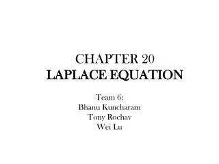
CHAPTER 20 LAPLACE EQUATION
CHAPTER 20 LAPLACE EQUATION. Team 6: Bhanu Kuncharam Tony Rochav Wei Lu. 20.1 Introduction. Remembering from chapter 16, the Laplacian operator (in Cartesian coordinates ): There are two types of Laplacian equations, Homogeneous

CHAPTER 20 LAPLACE EQUATION
E N D
Presentation Transcript
CHAPTER 20LAPLACE EQUATION Team 6: Bhanu Kuncharam Tony Rochav Wei Lu
20.1 Introduction Remembering from chapter 16, the Laplacian operator (in Cartesian coordinates): There are two types of Laplacian equations, • Homogeneous • Non-homogeneous (also known as the Poisson equation): Where f is a “source” function that is prescribed over the region in question.
Introduction A question to ask before we start going deeper into learning how to solve the Laplace equation is: Does this equation come up naturally? The answer to this question is yes. Let it be illustrated from the following example. Let’s consider the heat equation: Under which considerations would the Laplace equation arise? • Steady state (solution at equilibrium) • No heat sources Under these conditions the Laplace equation arises from physical situations.
20.2 Separation of Variables: Cartesian Coordinates The method of separation of variables assumes that the solution for an equation of multiple variable can be describes as the product of functions of a single variable. One function for each variable. For example. This method of solution can be applied to the Laplace equation when we assume that the Laplacian applies to a 2 dimensional function. How we solve Laplace’s equation will depend upon the geometry of the 2-D object we are solving it on.
y T=f2(x) H T=g1(y) T=g2(y) x 0 T=f1(x) L Separation of Variables Let’s start out by solving it on the rectangle given by 0 ≤ x ≤ L , 0 ≤ y ≤ H . For the geometry shown in the right, Laplace’s equation along with the four boundary conditions will be: • First notices that we don’t need and initial condition for this heat problem since the Laplace equation is homogeneous, meaning it is equal to zero, which is the equivalent of assuming a steady state for the T variable. • Next, let’s notice that while the partial differential equation is both linear and homogeneous the boundary conditions are only linear and are not homogeneous. This creates a problem because separation of variables requires homogeneous boundary conditions.
+ + T3(x,H)= f2(x) T2(x,H)=f2(x) T2(x,H)=0 T1(x,H)=0 T4(L,y)=g2(y) T1(L,y)=0 T3(L,y)=0 =g2(y) T2(L,y)=g2(y) T3(0,y)=g1(y) T1(0,y)=0 T3(0,y)=0 T2(0,y)=0 = T4(x,H)=0 T1(x,0)=f1(x) T3(x,0)=f1(x) T1(x,0)=f1(x) T2(x,0)=0 T4(L,y)=0 T4(0,y)= g1(y) + T4(x,0)=0 Separation of Variables To completely solve Laplace’s equation we are going to have to solve it four times. Each time we solve it only one of the four boundary conditions can be nonhomogeneous while the remaining three will be homogeneous. Because we know that Laplace’s equation is linear and homogeneous and each of the pieces is a solution to Laplace’s equation then the sum will also be a solution.
Separation of Variables Now, once solved all four of these problems the solution to our original system, (16), will be, Also, this will satisfy each of the four original boundary conditions. For example: And so on for the remaining boundary conditions. We will solve the problem in the following way: • Apply separation of variables to the each problem and find a product solution that will satisfy the differential equation and the three homogeneous boundary conditions. • Use the Principle of Superposition to find a solution to the problem and then apply the final boundary condition to determine the value of the constant(s) that are left in the problem. Two of the cases will be shown here and the two can be done as an additional exercise.
T2(x,H)=f2(x) T3(x,H)= f2(x) T2(x,H)=0 T1(x,H)=0 y T3(L,y)=0 =g2(y) T2(L,y)=g2(y) T1(L,y)=0 T4(L,y)=g2(y) T3(0,y)=0 T2(0,y)=0 T3(0,y)=g1(y) T1(0,y)=0 T4(x,H)=0 T3=f2(x) T1(x,0)=f1(x) T3(x,0)=f1(x) T1(x,0)=f1(x) T2(x,0)=0 H T4(L,y)=0 T4(0,y)= g1(y) T3=0 T3=0 T4(x,0)=0 x 0 T3=0 L Separation of Variables - Example 1 Find the solution to the following differential equation. Boundary Conditions: Notice that this example is a part of our original problem solution, it would be the third component of our solution. + = + +
y T3=f2(x) H T3=0 T3=0 x 0 T3=0 L Separation of Variables – Solution to Example 1 We assume the solution can be solved by separating the variable. In other words the solution can be expressed in the form: Our homogeneous boundary conditions now become: Next, we’ll plug the product solution into the differential equation.
Separation of Variables – Solution to Example 1 At this point we need to select our separation variable. We need identify were the two homogeneous boundaries exist and select the positive or negative variable that will give us a solution in the form of sine and cosine. After that you can find that how to build up the solution is different from one book to another. While in the textbook tend to find and combine all the solutions (using the superposition principle), others notice when only the positive or negative solution are non-trivial, thus reducing the need of working out so many constants In this section both approaches are exemplified, for the first two examples we eliminated the possibility of =0, integration constant being zero, because we know the values of all four boundary conditions.
Separation of Variables – Solution to Example 1 For the reasons mentioned before, for this case, we select our integration constant as (-). So, after adding in the separation constant we get, and two ordinary differential equations that we get from this case (along with their boundaryconditions) are, and
Separation of Variables – Solution to Example 1 Using our first ODE we find that the solution is, as intended, in the form: Applying the first boundary condition gives Applying the second boundary condition, and C1=0 to F(x) we get: Now, we after disregarding, trivial solutions, this means we must have:
Separation of Variables – Solution to Example 1 The positive eigenvalues and their corresponding eigenfunctions of this boundary value problem are then, The second differential equation is then, Because the coefficient of G is positive we know that a solution to this is, or
Separation of Variables – Solution to Example 1 Applying the boundary condition the solution becomes, The product solution for this case becomes, and solution to this partial differential equation is then,
Separation of Variables – Solution to Example 1 Finally, let’s apply the nonhomogeneous boundary condition to get the coefficients for this solution. As expected, this is again a Fourier sine series and so using previously done work instead of using the orthogonally of the sines to we see that,
Separation of Variables – Solution to Example 1 Finally we see that the solution for this problem is: Where • Important remarks:For the Laplace equation, the sign of the separation constant and the sequencing of the boundary conditions needs to be decided on a case-by-case basis. However the following rule of thumb can be used as guidance: “Anticipating the edge along which the eventual Fourier series will take place, chose the or - so as to obtain oscillatory functions along that edge. Then apply the boundary conditions adjacent to that edge first”.
Separation of Variables – Visualization of Example 1 Consider f(x), to be a constant, say f(x)=100Cand our rectangular body to have dimensions L=200, H=100. In this case, we can see the boundary conditions taking place in the eastern, western, and southern boundary were T=0. http://dylanh.bol.ucla.edu/CA/temperature.html
T3(x,H)= f2(x) T2(x,H)=f2(x) T1(x,H)=0 T2(x,H)=0 T3(L,y)=0 =g2(y) T4(L,y)=g2(y) T1(L,y)=0 T2(L,y)=g2(y) T3(0,y)=g1(y) T3(0,y)=0 T1(0,y)=0 T2(0,y)=0 T4(x,H)=0 T4(x,H)=0 T2(x,0)=0 T1(x,0)=f1(x) T3(x,0)=f1(x) T1(x,0)=f1(x) T4(L,y)=0 T4(L,y)=0 T4(0,y)= g1(y) T4(0,y)= g1(y) T4(x,0)=0 T4(x,0)=0 Separation of Variables – Example 2 Find a solution to the following PDE Boundary conditions: Notice that this example is a part of our original problem solution, it would be the fourth component of our solution. + = + +
Separation of Variables – Solution to Example 2 We start from assuming the solution can be solved by separating the variable. Boundary conditions: Next, we plug the product solution into the differential equation.
Separation of Variables – Solution to Example 2 At this point we need to choose a separation constant, in this case (), Note how the selection of this variable depends on where we have two boundary conditions. So, after adding in the separation constant we get, and two ordinary differential equations that we get from this case (along with their boundaryconditions) are and
Separation of Variables – Solution to Example 2 This time our second ODE has the sine, cosine, solution: Applying our boundary conditions we get to determine that The positive eigenvalues and their corresponding eigenfunctions of this boundary value problemare then,
Separation of Variables – Solution to Example 2 The second differential equation is then, Because the coefficient of F is positive we know that a solution to this is, However, this is not really suited for dealing with the h(L)= 0 boundary condition. So, let’s also notice that the following is also a solution: This is usually called a “shifted solution” and is very useful!
Separation of Variables – Solution to Example 2 Applying the lone boundary condition to this “shifted” solution gives, The solution to the first differential equation is now, And this is all the farther we can go with this because we only had a single boundary condition.That is not really a problem however because we now have enough information to form the product solution for this partial differential equation.A product solution for this partial differential equation is,
Separation of Variables – Solution to Example 2 The solution to this partial differential equation is then, Finally, let us apply the non-homogeneous boundary condition to get the coefficients for this solution. Now, in the previous problems we have done this has clearly been a Fourier series of some kind and in fact it still is. The difference here is that the coefficients of the Fourier sine series are now,
Separation of Variables – Solution to Example 2 Rememberthat a Fourier sine series is a series of coefficients (depending on n) times a sine.We still have that here, except the “coefficients” are a little messier this time that what we saw when we first dealt with Fourier series. So, the coefficients can be found using exactly the same formula from the Fourier sine series section of a function on 0 < y < H we just need to be careful with the coefficients.
Separation of Variables – Solution to Example 2 Finally we see that the solution for this problem is: Where
T2(x,H)=0 T3(x,H)= f2(x) T1(x,H)=0 T2(x,H)=f2(x) T3(L,y)=0 =g2(y) T1(L,y)=0 T2(L,y)=g2(y) T4(L,y)=g2(y) T1(0,y)=0 T2(0,y)=0 T3(0,y)=0 T3(0,y)=g1(y) T4(x,H)=0 T3(x,0)=f1(x) T2(x,0)=0 T1(x,0)=f1(x) T1(x,0)=f1(x) T4(L,y)=0 T4(0,y)= g1(y) T4(x,0)=0 Separation of Variables – Closing of Examples 1&2 Until this point we have worked two of the four cases (T3 &T4)that would need to be solved in order to completely solve the Laplace equation with non-homogenous boundary conditions in all four sides. As we have seen each case was similar and yet also had some differences. We saw the use of both separation constants and that sometimes we need to use a “shifted” solution in order to deal with one of the boundary conditions. The remaining cases can be easy to find after this explanation. + = + + The figure on the right illustrates the solution of the Laplace equation with non-homogeneous boundary conditions for al four sides, in this case fixed temperature in all four sides a square body such as the one in the problem. http://tigger.uic.edu/~rkodama/
y T=50 T=20 x 0 T=f(x) 5 Separation of Variables –Example 3 Consider the Dirichlet problem: With the Boundary Conditions:
Separation of Variables –Example 3 This example can very well represent a complicated three dimensional domain. Take for example the following figure from Greenberg’s book: Suppose that our interest is finding the temperature of the object near the end of the fin, within the rectangle ABCE, assume we don’t know the boundary along AB and the boundaries T=20 along AE, T=50 along BC, and T=f(x) along EC. To a good approximation, we render the problem tractable by letting D be the entire semi-infinite strips shown for the Dirichlet problem. Fig. Cooling fin* *Greenberg, M. D. (1998). Advanced Engineering Mathematics (2nd ed.): Prentice Hall.
Separation of Variables –Solution of Example 3 We assume the solution can be solved by separating the variable. In other words the solution is in the form: We apply this to the homogeneous boundary conditions first since we’ll need those once we get reach the point of choosing the separation constant. The boundary conditions become, Next, we plug the product solution into the differential equation.
Separation of Variables –Solution of Example 3 Now, at this point we need to choose a separation constant, in this case (-) So, The possible solutions to this ODEs are:
Separation of Variables –Solution of Example 3 This ODE has three types of equations, lets superimpose all the types of solutions. This will give: If we try to apply the boundness condition (y→∞) we note that the term y and the positive exponential will grow to infinite. Since this is not possible it is necessary that C6 =0and C7=0. This reduces our equation to: Grouping the constants:
Separation of Variables –Solution of Example 3 Now, the boundary condition in the left side: Matching the coefficients of the K1 and exp() terms on both sides of our previous equation gives K1= 20 and K3=0. Using this result, and updating T(x,y) we get: Next, we use the boundary condition at the right side: So Give
Separation of Variables –Solution of Example 3 Using this result to update T(x,y): This is the solution to our problem. Now we only need to find the value of Kn. To do this we use the lower boundary condition: Wefindthat or
Separation of Variables –Solution of Example 3 Applying the Fourier sine series we can find Kn as: Which is the constant that was missing to obtain the result of the Temperature in our semi-infinite slab equation:
20.3.1 Plane polar coordinates From figure polar coordinates can be written in terms of Cartesian coordinates 20.3 Separation of variables; Non-Cartesian Coodinates y r r sinθ θ r cosθ The laplacian in terms of polar coordinates where r, θ are independent variables which is same as equation (24) from section 16.7 x
Example 1: Direchlet Problem Problem definition: Physical Interpretation: The variable ‘u’ used here can be physically interpreted as temperature (T) in heat transfer problem Or concentration (C) in diffusion problem. The problem at hand can be seen as a temperature or concentration distribution in a cylindrical disk where the disk thickness is ‘z’, which is ignored (the temperature gradient in ‘z’ direction). u=f(θ) u=u2 u=0 r α θ a b u=u1
Solution using separation of variables method We seek solution in the form of Using this as solution the laplacian equation transforms into: Which can be simplified r and divide by RΘ to separate the variables Here +κ2 is chosen to obtain solution in the form of cosκθ and sinκθ instead of coshκθand sinhκθ since we anticipate that to satisfy the u(b,θ)=f(θ) boundary condition we need to expand f(θ) in a Fourier series (discussed later sections)
The previous differential equation can be written in a more familiar form as The solution can be written as: and Superposition of these two solutions (8a, 8b), we can write a general solution as Note: A, B, C,D E,F, G, H are arbitrary integration constants and needs to be evaluated.
Apply boundary conditions When θ=0 Set AE=u1 , B=0, and G=0 which gives When θ=α So u1+Iα=u2 and sinkα=0 gives u=f(θ) u=u2 u=0 r Boundary conditions α θ a b u=u1
We can write the solution after substituting equation 13a, 13b Using next boundary condition: Which can be written as: Where
Using next boundary condition: Which can be written as: Similar to previous expansion
Integrals in Equations (17) and (19) can be evaluated when f(θ) is specified which allows us to render them into algebraic equations. They can be solved to obtain a unique solution because the determinant matrix of coefficients is not zero. Numerical Example: Temperature distribution
Solution: Using the general solution from previous derivation Apply boundary conditions in above equation Evaluate Pn and Qn by solving the algebraic equations below: and
Solving above algebraic equations we get Final solution for temperature distribution in disk is given by following equation
20.3.2 Cylindrical coordinates z r θ b Z=0 Z=L The laplacian in terms of polar coordinates where r, θ,z are independent variables
Applying operator to a potential function and set it to zero, ignoring the source term. Assuming solution of the form and applying method of separation of variables Substituting equation (3) in equation (2) we get
Simplify by dividing by and use short hand notation for brevity Or separating ‘Z’ term Equations for the three components of solution can be written as follows For “Z” component
For “θ” component For “R” component Equation (7.3) is also known as Bessele Equation Solutions for equations (7.1), (7.2) is well known and
Solution to equation (7.3) is little more complicated, we will it find case by case below The solution to the equation that is regular at origin is • http://planetmath.org/encyclopedia/LaplaceEquationInCylindricalCoordinates.html (2) http://www.owlnet.rice.edu/~hill/phys532/L1b.pdf (3) Arfken, George, Weber, Hans, Mathematical Physics. Academic Press, San Diego, 2001 The solution is in terms of bessel function… Jv(kr) Case 1: kr<<1 Case 1: kr>>1 References