Download

1 / 47
470 likes | 496 Vues
Learn about the Union-Find data structure with constant time deletions, its applications in various algorithms, and the efficient handling of deletions. Understand how to maintain equivalence relations, compute minimum spanning trees, and more. Explore techniques for implementing meldable priority queues and computing minimum directed spanning trees. Discover the theoretical analysis behind amortized costs and the efficient implementation of delete operations. Dive deep into the concept of Union-Find without deletions, worst-case scenarios, and strategies for handling deletions effectively. Uncover methods for maintaining tidy and reduced trees, achieving deletions in constant time, and optimizing find operations.

E N D
Union-Find with Constant Time Deletions Stephen Alstrup Inge Li Gørtz Theis Rauhe Mikkel Thorup Uri Zwick
Union-Find • Make(x): Create a set containing x • Union(A,B): Unite the sets A and B • Find(x): Return the set containing x • Delete(x): Delete x from its set
Applications of Union-Find • Maintaining an equivalence relation • Computing minimum spanning trees • Computing dominators in graphs • Many other algorithms
Applications of Union-Find with deletions • Implementation of meldable priority queues • Meldable priority queues used to compute minimum directed spanning trees
Union-Find without deletions Worst case Smid ’90 Amortized Tarjan ’75
Amortized analysis [Tarjan ’75] [van Leeuven, Tarjan ’84] The cost of any intermixed sequence containing nmake operations and m find operations is O( n + mα(m+n,n) ) . [Kaplan, Shafrir, Tarjan ’02] The amortized cost of each find operation is only α(m+n,n,l), wherelis the number of operations in the set found.
Ackermann’s function A0(j) = j+1 Ai(j) = Ai-1(j+1)(j) Grows extremely FAST α(n) = min{ k : Ak(1) ≥ n } α(m,n) = min{ k : Ak(m/n) ≥ n } Grows extremelyslow
Union-Find with deletions [Kaplan, Shafrir, Tarjan ’02] Delete operations are not more expensive than find operations. They can thus be implemented in O(log l) worst case time and O(α(m+n,n,l)) amortized time. [Here] Delete operations can be implemented in O(1) worst case and amortized time.
Union Find Represent each set as a rooted tree Union by rank Path compression x The parent of a vertex x is denoted by p[x] Find(x) traces the path from x to the root
Union by rank r+1 r r2 r r1 0 r1< r2 Union by rank on its own gives O(log l) find time A tree of rank k contains at least 2k elements If x is not a root, then rank(x)<rank(p[x])
Handling deletions Simplest thing to do: Ignore them! Space O(N) instead of O(n),find time O(log N) instead of O(log l), where N is the # of elements ever created. Next thing to do: Global Rebuilding Keep track of the number of elements that were deleted. If at least, say, half of the elements are deleted, rebuild all trees. Easily works in the amortized setting.Can be done in the “background”.Find time is O(log n) or O(α(m+n,n)).
Handling deletions [Kaplan, Shafrir, Tarjan ’02] Local rebuilding • For each set keep an old tree and a new tree. • When an element is deleted from the old tree, move four elements to the new tree. • At least ¼ of the elements of the old tree are not deleted and at least ½ of the elements of the new tree are not deleted. • When the old tree is empty, the new tree takes its place and a new new tree is constructed. For each delete we need to do a find to know from which tree the element is deleted
Deletions in constant time • Keep trees tidy. • Following each delete, and in some other cases, perform a constant number of short-cut operations. Works in both the worst case and amortized settings
Tidy and untidy trees Nodes are either occupied or vacant • A tree is tidy if: • Every leaf is occupied and has rank 0. • Every vacantnon-root node has at least two children. At least ½ of the nodes of a tidy tree are occupied.
Reduced trees A reduced tree is a tidy tree of height 1whose root is of rank 1.
y y y z z x z Deleting an element from a tidy tree Remove the element from its node. If a leaf is now vacant, remove it from the tree. If a new leaf is created, reduce its rank to 0. If a vacant non-root element with only one child is created, short-cut it. y x z
Keeping tidy trees shallow After each deletion, perform sevenshort-cutting steps: Short-cut(v): “Take a grandchild of v and hang it on v” v Each short-cutting step is slightly more complicatedbut is still quite simple and takes only constant time.
v v short-cut(v) Case 1: v has an occupied child which has a child
v v short-cut(v) Case 2: v has a vacant child with at least three children
v v short-cut(v) Case 3: v has a vacant child with two occupied children
v v short-cut(v) Case 4: v has a vacant grandchild with at least three children
v v short-cut(v) Case 5: v has a vacant grandchild with only two children
short-cut(v) Case 6: If v does not have grandchildren,let v←p[p[v]] and try again Case 7: If v does not have grandchildren and is a root, change the rank of v to 1. The tree is now reduced.
The trees are shallow Theorem:|A| ≥ (2/3)(6/5)rank(A) Corollary: rank(A) ≤ log6/5(3|A|/2) = O(log|A|+1) Find takes O(log l) worst-case time
Values Value of a node x : (5/3)rank(p[x]) if x occupied val(x) = (1/2)(5/3)rank(p[x]))if x vacant Value of a set A : VAL(A) = ∑xA val(x) Theorem: VAL(A) ≥ 2rank(A)
VAL(A) ≥ 2rank(A) Show that a delete operation, followed by four short-cutting steps, either does not decrease the value, or generates a reduced tree. It is easy to show that make and union maintain this property Later we will show that this property is also maintained by path compression, with an appropriate collection of short-cuts
|A| ≥ (2/3)(6/5)rank(A) The tree representing A contains exactly |A| occupied nodes and at most |A| vacant nodes (3/2) |A| (5/3)rank(A) ≥ VAL(A) ≥ 2rank(A) |A| ≥ (2/3)(6/5)rank(A)
How much value is lost by delete? k=rank[v] v v y x z z Value lost: –(5/3)k-1 – (1/2)(5/3)k + (1/2)( (5/3)k–(5/3)k-1 )= (9/10)(5/3)k
v v short-cut(v) Case 1: v has an occupied child which has a child Gain: (1/2)((5/3)k-(5/3)k-1) = (1/5)(5/3)k
v v short-cut(v) Case 2: v has a vacant child with at least three children Gain: (1/2)((5/3)k-(5/3)k-1) = (1/5)(5/3)k
v v short-cut(v) Case 3: v has a vacant child with two occupied children Gain: 2((5/3)k-(5/3)k-1) – (1/2)(5/3)k = (3/10)(5/3)k
v v short-cut(v) Case 4: v has a vacant grandchild with at least three children Gain: (1/2)((5/3)k-(5/3)k-2) = (8/25)(5/3)k
v v short-cut(v) Case 5: v has a vacant grandchild with only two children Gain: (1/2)((5/3)k–(5/3)k-2) + (1/2) ((5/3)k-1–(5/3)k-2) – (1/2)(5/3)k-1 = (7/50)(5/3)k
Amortized bounds • Path compression and shortcutting combine nicely together. • After each path compression we need to do some tidying up and some short-cuts to maintain the value • Give new potential-based analysis for local amortized bounds. x
Melding Priority Queues Ran Mendelson Robert E. Tarjan Mikkel Thorup Uri Zwick
Improved analysisof transformation MeldablePriority Queue Non-meldablePriority Queue pq(n)+α(n) timeper operation pq(n) timeper operation or pq(n)α(n,n/pq(n)) timeper operation
Second transformation MeldablePriority Queue pq(n) timeper operation pq(N) timeper operation n – number of elements in priority queue Keys are is {1,2,…,N}
Meldable Priority Queues Insert Delete Find-Min O(1) O(log n) O(1) O(1) 10 25 4 7 2 13 17 1 O(1) Dec-Key 5 38 Meld Amortized[Fredman-Tarjan ’87] Worst case[Brodal ’96] Best possible comparison based results
RAM Priority Queues Keys are integers that fit into a single machine word.Standard arithmetical and logical operations take constant time Insert Delete Find-Min O(1) O(log log n) O(1) O(1) 010010 001001 011010 Dec-Key using our transformation Meld O(1) NO [Thorup ’03]
Atomic heaps Insert Delete Find-Min O(1) O(1) O(1) 011010 000010 010011 At most O(log2n) elements! Meld NO [Fredman-Willard ’94]
Non-meldable priority queue+Union Find with deletions Meldable priority queue
Use the union-find data stricture to maintain the sets Place a non-meldable priority queue at each node of a union-find tree holding the minimal element in each one of its subtrees 9 1 5 1 2 4 5 3 19 2 7 4 8 6 19 2 4 8 6
Handling deletions using path compression The amortized delete cost is O(pq(n)α(n)) [MTZ’04] [van Emde Boaz, Kaas, Zijlstra ’77 ]
Flavor of improved analysis rank ≥ k At mostn/2k nodes size ≥ 2k rank < k size < 2k Choose k=2loglog n. If f>n/log n, we are done.
More flavor of improved analysis rank ≥ k size ≥ 2k rank < k size ≥ 2k rank < k size < 2k
Sorting Worst-case non-meldable priority queues Amortized meldablepriority queues