Hypothesis Testing:
Hypothesis Testing:. Inferential statistics. These will help us to decide if we should:. 1) believe that the relationship we found in our sample data is the same as the relationship we would find if we tested the entire population. OR.


Hypothesis Testing:
E N D
Presentation Transcript
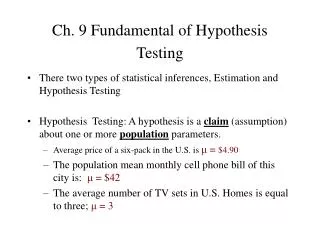
Inferential statistics These will help us to decide if we should: 1) believe that the relationship we found in our sample data is the same as the relationship we would find if we tested the entire population OR 2) believe that the relationship we found in our sample data is a coincidence produced by sampling error
Inferential statistics • Univariate statistical analysis: tests hypotheses involving only one variable • Bivariate statistical analysis: tests hypotheses involving two variables • Multivariate statistical analysis: tests hypotheses and models involving multiple variables
Specific Steps in Hypothesis Testing • Specify the hypothesis. • Select an appropriate statistical test. • Two-tailed or One-tailed test. • Specify a decision rule (alpha = ???). Compute the critical value. • Calculate the value of the test statistic and perform the test. • State the conclusion.
Hypotheses and statistical tests In general, when you make a testable hypothesis, you specify the relationship you expect to find between your IV and the DV. If you specify the exactdirection of the relationship (i.e., longer math tests will increase test anxiety), then you will perform a 1-tailed test. At other times, you may not know or predict a specific result direction but rather just that performance will change (ie. longer math tests will affect test anxiety), then you will perform a 2-tailed test.
Hypothesis • NULL Hypothesis: world view or Status quo. • Alternative Hypothesis: Researcher’s theory • -H0 The average age of a large class is 25. • -H1 The average age of a large class is different than 25 (two tail) • - H1 The average age of a large class is less than 25. • Other examples?
The One-sample Experiment This is a pretty high score. It’s lower than the industry average, but it is “within range.” Based on this one score can I say that X’s score is significantly, different than industry score? Let’s say you know the value of a particular characteristic in the population (this is uncommon) - i.e., Computer Industry Satisfaction is normal (mean=100, SD=15) It turns out that we have one CS score for a company X(X = 84)
Statistical Hypotheses (1-tailed) Alternative hypothesis (H1): x < i Null hypothesis (H0): xi H1: X has CS lower than industry H2: X has an equal to or greater CS than industry Given: i = 100
Statistical Hypotheses (2-tailed) Alternative hypothesis (H1): x ≠ I Null hypothesis (H0): x = i H1: X has different CS than industry H2: X has an equal CS to industry Given: i = 100
Logic of Statistical Hypothesis Testing We measured CS on a sample of companies (for the moment N=1) and find that mean CS for the sample of companies is less than the industry mean of 100. Does this mean that X has lower CS? Or , the possible explanations are: X indeed has lower CS 2) X has the same CS, but sampling error produced the smaller mean CS score. We could run everyone in the population (not possible), or use inferential statistics to choose between these two alternatives.
Logic of Statistical Hypothesis Testing The logic goes like this: Inferential statistics will tell us how likely it would be to get a sample mean like the one we measured given that the null hypothesis (H0) is true. If it is really UNlikely that we would get a mean score like we did, drawing a sample from the population of the x = 100), then we conclude that our sample did not come from that population, but from a different one. We reject the null hypothesis.
Logic of Statistical Hypothesis Testing All statistical tests use this logic: - determine the probability that sampling error (random chance) has produced the sample data from a population described by the null hypothesis (H0). Let’s look at the z-test to see how this works.
Assumptions of the z-test • We have randomly selected one sample (for the moment N=1) • The dependent variable is at least approximately normally distributed in the population and involves an interval or ratio scale • We know the mean of the population of raw scores under some other condition of the independent variable • We know the true standard deviation of the population sxdescribed by the null hypothesis
Before you compute the test statistic • Choose your alpha () level, the criterion you will use to determine whether to accept or reject H0, .05 is typical in psychology/mkt/mgm • Identify the region of rejection (1- or 2-tailed) • Determine the critical value for your statistic • - for z-test, the critical value is labeled zcrit
2-tailed regions A sampling distribution for H0 showing the region of rejection for a = .05 in a 2-tailed z-test.
1-tailed region, above mean A sampling distribution for H0 showing the region of rejection for a = .05 in a 1-tailed z-test.
1-tailed region, below mean A sampling distribution for H0 showing the region of rejection for a = .05 in a 1-tailed z-test where a decrease in the mean is predicted.
Finding zcrit (2-tailed) To find zcrit, we will use our z-table to find the z-score that gives us the appropriate proportion of scores in the region of rejection (in the tails of the distribution).
Finding zcrit (1-tailed) To find zcrit, we will use our z-table to find the z-score that gives us the appropriate proportion of scores in the region of rejection (in the tails of the distribution).
Computing zobt for the test zobt = 84 - 100 = 16 = -1.07 15 15 You calculate the z-score for your sample mean in a similar way as we did for a single score and it is labeled zobt. SEM: What does it mean?
Interpreting zobt relative to zcrit You then compare your zobtvalue tothe zcritvalue. If zobtis beyond zcrit(more into the tail of the distribution), then we will say that we “reject the null hypothesis”. 2-tail 1-tail Note: in this case we fail to reject the null hypothesis. This does not mean the null is true. Indeed, in this case it is almost certainly not true. Don’t forget this it is really important!!! We then report that our results were “notsignificant” or “nonsignificant” and report it like this: z = +1.07, p > .05
Now suppose that we have a sample of 3 companies CS scores. SO, and
Interpreting zobt relative to zcrit You then compare your zobtvalue tothe zcritvalue. If zobtis beyond zcrit(more into the tail of the distribution), then we will say that we “reject the null hypothesis”. 2-tail 1-tail As a logical consequence, if we have rejected the null hypothesis then we have supported the alternative hypothesis. BUT we have not PROVED anything. We then report that the difference was “statistically significant” and report it like this: z = -1.86, p < .05
Errors Since our statistical procedures are based on probabilities, there is a possibility that our data turned out as they did from chance alone. Type I: rejecting the null hypothesis when it is actually true, the probability of making this error is equal to , our chosen criterion. Type II: accepting the null hypothesis when it is actually false, the probability of making this error can be computed and it is labeled .
The One-sample t-test We rarely know the population characteristics, particularly the SD, and thus we rarely use the z-test. If we know the population mean, but not the SD, we must use the t-test rather than the z-test. The logic is identical.
Assumptions of the t-test • We have randomly selected one sample • The dependent variable is at least approximately normally distributed in the population and involves an interval or ratio scale • We know the mean of the population of raw scores under some other condition of the independent variable • We do notknow the true standard deviation of the population described by the null hypothesis so we will estimate it using our sample data.
Before you compute the test statistic • Choose your alpha () level, .05 is common • Identify the region of rejection (1- or 2-tailed) • Determine the critical value for your statistic • - for t-test, the critical value is labeled tcrit
Computing tobt for the test You calculate tobt for your sample mean in a similar way as we did for zobt.
Compare tobt relative to tcrit As with the z-test, for the t-test you will compare tobtto tcrit. So how do you find tcrit? You look in a table of the t-distribution. The t-distribution contains all possible values of t computed for random sample means selected from the population described by the null hypothesis (similar to the z-distribution). One BIG difference, is that there are many t-distributions for any population, one for every sample size. As N increases, the t-distribution better approximates a normal distribution, until N ~ 120.
Finding tcrit Since there are different t-distributions for different sample sizes, we must find tcrit from the appropriate t-distribution. The appropriate t-distribution will be the one that matches our sample size, which we now call degrees of freedom (df). For the t-test, the degrees of freedom equals N-1, When N-1 is more than 120, the t-distribution is indistinguishable from a true normal distribution and thus use df=.
Finding tcrit (2-tailed) To find tcrit, use the t-table to find the t for the df that corresponds to your sample size (N-1) for the criterion () you have chosen.
Finding tcrit (1-tailed) To find tcrit, use the t-table to find the t for the df that corresponds to your sample size (N-1) for the criterion () you have chosen.
Interpreting tobt relative to tcrit If tobtis less than tcrit(away from the area of rejection), then we will say that we “failed to reject the null hypothesis”. We then report that our results were “not significant” or “nonsignificant” and report it like this: t (2) = 1.86, p > .05
Modification of calculation when we compare means of two different samples What is the null? The alternative?
Chi-Square Test Requirements 1. Quantitative data. 2. One or more categories. 3. Independent observations. 4. Adequate sample size (at least 10). 5. Simple random sample. 6. Data in frequency form. 7. All observations must be used Think of types of research questions that can be answered using this test
How do you know the expected frequencies? • You hypothesize that they are equal in each group (category) • Prior knowledge, census data
Color preference in a car dealership (univariate) Chi-square=26.95 With df=5-1=4