Efficient Indexing Strategies in Data Warehousing: Comparative Analysis
200 likes | 240 Vues
This chapter analyzes indexing strategies in Data Warehousing. Discusses tuple clustering, page clustering, secondary indexes, bit-map indexes, and multidimensional indexing. Concludes with performance comparisons.

Efficient Indexing Strategies in Data Warehousing: Comparative Analysis
E N D
Presentation Transcript
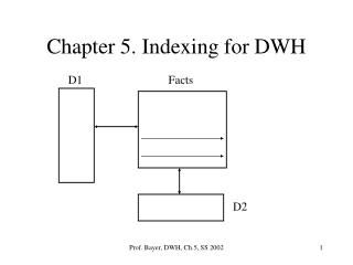
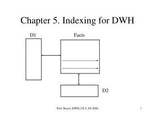
Chapter 5. Indexing for DWH D1 Facts D2 Prof. Bayer, DWH, Ch.5, SS 2000
dimension Time with composite key K1 according to hierarchy key K1 = (year int, month int, day int) dimension Region with composite key K2 according to hierarchy key K2 = (region string, nation string, state string, city string) Facts.key = (K1; K2) = KF create tableFacts ( measure real, ... ) key is (K1, K2) Prof. Bayer, DWH, Ch.5, SS 2000
Variant 1: Facts organized as compound B-tree, e.g. in TransBase (standard) or in Oracle as IOT: Index Organized Table i.e. data, measures are stored on leafs of tree and sorted according to lexicographic order of KF ==> Interval queries for K1 on D1 and on Facts ==> sorted reading according to lexicographic order of KF possible on Facts: tuple clustering!! ==> restrictions on K2 can be used on D2, but not on Facts Prof. Bayer, DWH, Ch.5, SS 2000
Variant 2: Full Table Scan (FTS) page clustering!! without any index support, works well , as soon as >10% of the data must be checked (retrieved from disk) to compute the answer this is an empirical observation with Oracle (similar in other rel DBMS) made with very large DBs ( > 1 GB) in the MISTRAL project Reason: random access 9 ms + page transfer 1 ms = 10 ms time (20 pages sequential) = 29 ms time (20 pages random ) = 200 ms factor 7 Prof. Bayer, DWH, Ch.5, SS 2000
Variant 3: Secondary indexes on Facts Problem: no tuple clustering and no page clustering!! create index SI (Facts, K1) create index SI (Facts, K2) select SI (Facts, c1) = list of ROWIDs select SI (Facts, c2) = list of ROWIDs, intersect select SI (Facts, i1) = list of list of ROWIDs for interval i1 = Set1 of ROWIDs select SI (Facts, i2) = list of list of ROWIDs for interval i2 = Set2 of ROWIDs Prof. Bayer, DWH, Ch.5, SS 2000
QueryBox ~ set of tuples with ROWID of Set1 Set2 This requires the following steps: 1. Sort Set1 2. Sort Set2 3. Compute intersection 4. For all ROWIDs r in intersection : fetch (Facts.r) ==> random access to disk for every tuple in answer Prof. Bayer, DWH, Ch.5, SS 2000
Speed Comparison: assumptions: 8 KB pages 50 tuples per page ~ 160 B/tuple disk parameters as before Variant 1: compound B-tree, tuple clustering: (10 ms/page)/(50 tuples/page) = 200 ms/tuple Variant 2: FTS, tuple clustering and page clustering: (29 ms/20 pages)/(50 tuples/page) = 29 ms/tuple Variant 3: secondary indexes, no clustering: (10 ms/page)/(1 tuple/page) = 10,000 ms/tuple Prof. Bayer, DWH, Ch.5, SS 2000
Conclusions • Tuple clustering gains factor 50 (depending on page and tuple size) over no clustering • Page and tuple clustering gains factor 345 over no clustering • Secondary indexes are a bad idea, except for point queries resulting in a single tuple !!! Prof. Bayer, DWH, Ch.5, SS 2000
Variant 4: Bit-Map indexes Facts with ROWIDs 1 2 ... k assume that attribute A has potential values a1, a2, a3, ..., alA BMI(A) is a set of Boolean vectors, one for each of a1, a2, a3, ..., alA BMI(A)[ai] = Boolean array BMI(A)[ai][1:k] BMI(A)[ai][j] = true iff Facts.j.A = aj false otherwise for ROWID j Prof. Bayer, DWH, Ch.5, SS 2000
1 2 … k BMI(A) = a1 a2 : aWA 0 1 0 … 0 1 1 0 1 … 0 Prof. Bayer, DWH, Ch.5, SS 2000
Note: in every column of BMI there is exactly one entry with value true ==> extremely sparse matrix, compression? Bitmaps: store rows of BMI in compressed form! Secondary indexes: entry for ai is the list of ROWIDs , which have true in row ai, usually sorted by ROWID, makes intersection more efficient, avoids additional sorting. Prof. Bayer, DWH, Ch.5, SS 2000
Queries: A = VAand B = VB ==> BMI(A)[VA] and BMI(B)[VB] yields set of ROWIDs r with Facts.r.A = VAand Facts.r.B = VB ==> these ROWIDs are already sorted and the tuples may be read pseudosequentially from the disk ==> for small result sets this requires 1 page access per result tuple, very slow, factor 50 slower compared to tuple clustering, see later performance results in chapter 6, 7, 8. Prof. Bayer, DWH, Ch.5, SS 2000
Note: bit map indexes and secondary indexes are very similar: • Bit map: representation of BMI as Boolean vector • Secondary index: representation of BMI as list of those ROWIDs with entry true • column representation ~ enumeration type Prof. Bayer, DWH, Ch.5, SS 2000
Variant 5: multidimensional index on the Facts table • Grid-file • R-tree • R*-tree • UB-tree • Decisive aspects: see chapter on UB-trees • tuple clustering • page clustering • sorted reading and writing • utilizing all restrictions of the query box Prof. Bayer, DWH, Ch.5, SS 2000
Variant 6: Hash indexes • no tuple clustering • no page clustering • no sorted reading and writing • depends very much on quality of hash functions • utilizing all restrictions of the query box only with multiple hash indexes Prof. Bayer, DWH, Ch.5, SS 2000
Variant 7: Join-Indexes Idea: partial materialization of a view for a join R joinA S starting point are SI(R,A) and SI(S, A) SI(R, a) = set of ROWIDs of relation R SI(S, a) = set of ROWIDs of relation S Join-Index JI (R, S, A): JI(R,S,a) = set of ROWID-pairs, whose tuples are join-partners. Prof. Bayer, DWH, Ch.5, SS 2000
Note: Result presentation with join-indexes requires 2 random accesses to R and S to produce 1 result tuple, very fast to produce the first result, additional results at about 50 tuples per second, faster than a person can read on the screen Note: in a join (R joinAS) the attribute A is usually a primary key of one involved relation (causing tuple clustering) and a secondary key in the other. Then sequential access with tuple clustering on one relation can be exploited, roughly doubles the performance. Note: In DWH applications the relation with the primary key is the dimension table and the relation with the foreign key is the fact table, therefore a slow solution. Prof. Bayer, DWH, Ch.5, SS 2000
Note: JI(R,S,A) „belongs“ to 2 relations, this causes a novel Index-Update-Problem, everytime either R or S are updated Question: Simulation of JI(R,S,A) by SI(R,A) and SI (S,A) and query-rewriting, i.e. optimization?? Prof. Bayer, DWH, Ch.5, SS 2000