Download

1 / 30
310 likes | 498 Vues
Flexible Budgets and Variances. Identifying Problems and Opportunities. Flexible Budgets. Standard Inputs required to get actual outputs. The Budget figure we would have used if we had known actual output in advance.

E N D
Flexible Budgets and Variances Identifying Problems and Opportunities
Flexible Budgets • Standard Inputs required to get actual outputs. • The Budget figure we would have used if we had known actual output in advance. • The flexible budget adjusts, after the fact, to give an expectation of what costs should have been for the actual output that we got.
Flexible Budget for Labor • Suppose that we normally use 3 labor hours for every unit that we produce and that we pay $10 per hour for labor. • If we plan on producing 100 units, our budget would be for 300 hours @ $10 per hour. • If we actually produced 80 units, our Flexible budget would be for 240 hours at $10 per hour
Flexible Budgets • In order to calculate the Flexible budget, it is necessary to know what actual output was. • It can only be calculated after we have completed the production for the year. • The flexible budget allows us to evaluate how efficiently we have used our inputs to produce our outputs.
Efficiency • Efficiency relates inputs to outputs. • We are more efficient if we get more output from a given amount of inputs or if we use less inputs for a given amount of output. • Effectiveness relates to the ability to accomplish a task or achieve a goal.
Variances • Variances compare actual results to budgeted results. • Variances highlight performance that is not in accordance with the budget and may require managerial attention. • Variances are either “favorable” or “unfavorable”. • Favorable variances generally result in income being higher than planned. • Unfavorable variances result in income being lower than planned.
Labor Price Variance • The Price or Rate Variance is caused by the actual wage being different from the standard wage. (P) • Price Variance = P * Qa • The “” term gives the variance its name. • Dollars per unit * Units = Dollars. • The quantity is the actual quantity.
Labor Efficiency Variance • The Efficiency or Quantity Variance is caused by the actual quantity of inputs being different from the standard quantity of inputs. (Q) • Quantity Variance = Q * Ps • Again, the“” term gives the variance its name. • Units * dollars per unit = dollars • The price is the standard price
Labor Variances - Example • Morgan Company generally uses 6 labor hours per unit at $12 per hour. They had planned to produce 5,000 units in October. • Morgan actually produced 6,000 units and used 38,000 hours paying $10 per hour.
Identification of Variables • Ps = $12 • Pa = $10 • Qa = 38,000 hours • Qs = 6 * 6,000 = 36,000 hours • Qs = standard inputs for actual outputs.
Calculation of Variances • Price Variance = P * Qa • = (12 - 10) * 38,000 • = $76,000 Favorable • Its favorable because it cost us less than standard. • Efficiency Variance = Q * Ps • =(38,000 - 36,000) * (12) • = $24,000 Unfavorable • Its unfavorable because we used more than we had planned for the output that we got.
Materials • What changes if we consider materials instead of labor? • Can we still get a price variance and an efficiency variance? • The only difference relates to Qa. • Is Qa the actual quantity purchased, or the actual quantity used in production?
Qa • The best Qa depends upon the variance we are calculating. • For the price variance, Qa is the quantity purchased, for the efficiency variance, Qa is the quantity used in production. • Other than this, the variances are calculated in the same way as for labor.
Materials Variances - Example • Morgan Company uses 8 pounds of materials for each unit they produce. They pay $6 per pound. They plan on producing 1,000 units in October. • During October, they actually produced 1,200 units. They used 10,000 pounds of materials. They purchased 9,000 pounds at $5 a pound.
Identification of Variables • Ps = $6 • Pa = $5 • Qused = 10,000 pounds • Qpurchased = 9,000 pounds • Qs = 8 * 1,200 = 9,600 pounds • Qs = standard inputs for actual outputs.
Calculation of Variances • Price Variance = P * Qpurchased • = (6-5) * 9,000 • = $9,000 Favorable • It is favorable because it cost less than expected • Efficiency Variance = Q * Ps • =(10,000 - 9,600) * (6) • = $2,400 Unfavorable • Its unfavorable because we used more than we had planned for the output that we got.
Overhead Variances • Overhead is separated into fixed and variable components before variances are computed. • There are two variable overhead variances and two fixed overhead variances.
Variable Overhead Variances • We use the same approach to variable overhead as we do for labor and materials. • We still calculate a price variance and an efficiency variance. • Sometimes the price variance is easier with a slightly different form of the equation.
Variable Overhead Price Variance • Price Variance = P * Qa • = (Ps- Pa) * Qa • = (Ps * Qa)- (Pa * Qa) • = (Ps * Qa)- VOHa • Ps is the variable overhead application rate
Observations of VOH Variances • If variable overhead is applied based upon labor hours, the Q’s for variable overhead will be the same as those for labor. • If variable overhead is applied based upon labor hours, the efficiency variances for labor and VOH will either both be favorable or both be unfavorable. • In any case, the Q for VOH is measured in terms of the allocation base or cost driver for VOH.
VOH Variances - Example • Morgan Company applies VOH based upon Direct labor hours. They generally use 6 labor hours per unit at $12 per hour and apply VOH at $6 per hour. • Morgan actually produced 6,000 units and used 38,000 hours. • Actual VOH was $247,000.
Identification of Variables • Ps = $6 • Qa = 38,000 hours • Qs = 6 * 6,000 = 36,000 hours • VOHa = 247,000 • Qs = standard inputs for actual outputs.
Calculation of Variances • Price Variance = (Ps * Qa)- VOHa • = (6 * 38,000) - 247,000 • = $19,000 Unfavorable • It is unfavorable because it cost more per hour than expected • Efficiency Variance = Q * Ps • =(38,000 - 36,000) * (6) • = $12,000 Unfavorable • Its unfavorable because we used more than we had planned for the output that we got.
Fixed Overhead Variances • There are 2 variances for fixed overhead, the spending variance and the volume variance. • The spending variance is similar to a price variance • The volume variance is similar to an efficiency variance.
Spending Variance • The spending variance is calculated by comparing the Actual Fixed overhead with the Budgeted Fixed Overhead. • If Actual is greater than Budgeted, it is Unfavorable. • If Actual is less than Budgeted, it is Favorable.
Volume Variance • The volume variance is calculated by comparing the fixed overhead applied to the fixed overhead budgeted. • It the applied is greater than the budgeted, it is favorable. (we got more output from a fixed input than we had expected) • It the applied is less than the budgeted, it is unfavorable. (we got less output from a fixed input than we had expected)
Fixed Overhead Variances - Example • Morgan Company estimates that they will produce 5,000 units during October and that their fixed overhead will be $90,000. • Morgan actually produced 6,000 units and had fixed overhead of $110,000. • Fixed Overhead is applied based upon labor hours, at 6 hours per unit.
Identification of Variables • Budgeted Fixed Overhead $90,000 • Actual Fixed Overhead $110,000 • Applied Fixed Overhead $108,000 • Applied = Qa * Std Hours per Unit * Application Rate • Applied = 6,000 * 6 * 3 • Application Rate = 90,000 / (5,000 * 6) = $3 per hour
Calculation of Variances • Spending Variance = Actual - Budget • = 110,000 - 90,000 • = $20,000 Unfavorable • Its unfavorable because it cost us more than standard. • Volume Variance = Budgeted - Applied • 90,000 - 108,000 • = $18,000 Favorable • Its favorable because we got more output than we had planned.