Download
1 / 57
600 likes | 918 Vues
Statistics for Business and Economics 9 th Edition. Chapter 10 Statistical Inferences About Means and Proportions with Two Populations. Two Sample Tests. Two Sample Tests. Population Means, Independent Samples. Population Means, Matched Pairs. Population Proportions. Interval

E N D
Statistics for Business and Economics9th Edition Chapter 10 Statistical Inferences About Meansand Proportions with Two Populations
Two Sample Tests Two Sample Tests Population Means, Independent Samples Population Means, Matched Pairs Population Proportions Interval Estimation Examples: Same group before vs. after treatment Group 1 vs. independent Group 2 Hypothesis Tests Proportion 1 vs. Proportion 2
Difference Between Two Means Population means, independent samples σx2 and σy2 known Test statistic is a z value σx2 and σy2 unknown 大样本 σx2 and σy2 assumed equal Test statistic is a a value from the Student’s t distribution 小样本 σx2 and σy2 assumed unequal
Difference Between Two Means Goal: Form a confidence interval for the difference between two population means, μx – μy • Different data sources • Unrelated • Independent • Sample selected from one population has no effect on the sample selected from the other population Population means, independent samples
σx2 and σy2 Known Population means, independent samples Assumptions: • Samples are randomly and • independently drawn • both population distributions • are normal • Population variances are • known * σx2 and σy2 known σx2 and σy2 unknown
Let equal the mean of sample 1 and equal the mean of sample 2. • The point estimator of the difference between the means of the populations 1 and 2 is . Estimating the Difference BetweenTwo Population Means • Let 1 equal the mean of population 1 and 2 equal the mean of population 2. • The difference between the two population means is 1 - 2. • To estimate 1 - 2, we will select a simple random sample of size n1 from population 1 and a simple random sample of size n2 from population 2.
Sampling Distribution of • Expected Value • Standard Deviation (Standard Error) where: 1 = standard deviation of population 1 2 = standard deviation of population 2 n1 = sample size from population 1 n2 = sample size from population 2
Interval Estimation of 1 - 2:s 1 and s 2Known • Interval Estimate where: 1 - is the confidence coefficient
Difference Between Two Means (continued) Population means, independent samples σx2 and σy2 known Test statistic is a z value σx2 and σy2 unknown 大样本 σx2 and σy2 assumed equal Test statistic is a a value from the Student’s t distribution 小样本 σx2 and σy2 assumed unequal
σx2 and σy2 Known Population means, independent samples Assumptions: • Samples are randomly and • independently drawn • both population distributions • are normal • Population variances are • known * σx2 and σy2 known σx2 and σy2 unknown
σx2 and σy2 Known (continued) When σx2 and σy2 are known and both populations are normal, the variance of X – Y is Population means, independent samples * σx2 and σy2 known …and the random variable has a standard normal distribution σx2 and σy2 unknown
Test Statistic, σx2 and σy2 Known Population means, independent samples The test statistic for μx – μy is: * σx2 and σy2 known σx2 and σy2 unknown
Interval Estimation of 1 - 2:s 1 and s 2Known • Interval Estimate where: 1 - is the confidence coefficient
Hypothesis Tests forTwo Population Means Two Population Means, Independent Samples Lower-tail test: H0: μxμy H1: μx < μy i.e., H0: μx – μy 0 H1: μx – μy< 0 Upper-tail test: H0: μx ≤ μy H1: μx>μy i.e., H0: μx – μy≤ 0 H1: μx – μy> 0 Two-tail test: H0: μx = μy H1: μx≠μy i.e., H0: μx – μy= 0 H1: μx – μy≠ 0
Decision Rules Two Population Means, Independent Samples, Variances Known Lower-tail test: H0: μ1 – μ2 0 H1: μ1 – μ2< 0 Upper-tail test: H0: μ1 – μ2≤ 0 H1: μ1 – μ2> 0 Two-tail test: H0: μ1 – μ2= 0 H1: μ1 – μy≠ 0 a a a/2 a/2 -za za -za/2 za/2 Reject H0 if z < -za Reject H0 if z > za Reject H0 if z < -za/2 or z > za/2
Interval Estimation of 1 - 2:s 1 and s 2 Known • Example: Par, Inc. Par, Inc. is a manufacturer of golf equipment and has developed a new golf ball that has been designed to provide “extra distance.” In a test of driving distance using a mechanical driving device, a sample of Par golf balls was compared with a sample of golf balls made by Rap, Ltd., a competitor. The sample statistics appear on the next slide.
Interval Estimation of 1 - 2:s 1 and s 2 Known • Example: Par, Inc. Sample #1 Par, Inc. Sample #2 Rap, Ltd. Sample Size 120 balls 80 balls Sample Mean 275 yards 258 yards Based on data from previous driving distance tests, the two population standard deviations are known with s 1 = 15 yards and s 2 = 20 yards.
Interval Estimation of 1 - 2:s 1 and s 2 Known • Example: Par, Inc. Let us develop a 95% confidence interval estimate of the difference between the mean driving distances of the two brands of golf ball.
Population 1 Par, Inc. Golf Balls m1 = mean driving distance of Par golf balls Population 2 Rap, Ltd. Golf Balls m2 = mean driving distance of Rap golf balls Simple random sample of n1 Par golf balls x1 = sample mean distance for the Par golf balls Simple random sample of n2 Rap golf balls x2 = sample mean distance for the Rap golf balls x1 - x2 = Point Estimate of m1 –m2 Estimating the Difference BetweenTwo Population Means m1 –m2= difference between the mean distances
Point Estimate of 1 - 2 Point estimate of 1-2 = = 275 - 258 = 17 yards where: 1 = mean distance for the population of Par, Inc. golf balls 2 = mean distance for the population of Rap, Ltd. golf balls
Interval Estimation of 1 - 2:1 and 2 Known 17 + 5.14 or 11.86 yards to 22.14 yards We are 95% confident that the difference between the mean driving distances of Par, Inc. balls and Rap, Ltd. balls is 11.86 to 22.14 yards.
Hypothesis Tests About m 1-m 2:s 1 and s 2 Known • Example: Par, Inc. Can we conclude, using a = .01, that the mean driving distance of Par, Inc. golf balls is greater than the mean driving distance of Rap, Ltd. golf balls?
Hypothesis Tests About m 1-m 2:s 1 and s 2 Known • p –Value and Critical Value Approaches 1. Develop the hypotheses. H0: 1 - 2< 0 Ha: 1 - 2 > 0 where: 1 = mean distance for the population of Par, Inc. golf balls 2 = mean distance for the population of Rap, Ltd. golf balls a = .01 2. Specify the level of significance.
Hypothesis Tests About m 1-m 2:s 1 and s 2 Known • p –Value and Critical Value Approaches 3. Compute the value of the test statistic.
Hypothesis Tests About m 1-m 2:s 1 and s 2 Known • p –Value Approach 4. Compute the p–value. For z = 6.49, the p –value < .0001. 5. Determine whether to reject H0. Because p–value <a = .01, we reject H0. At the .01 level of significance, the sample evidence indicates the mean driving distance of Par, Inc. golf balls is greater than the mean driving distance of Rap, Ltd. golf balls.
Hypothesis Tests About m 1-m 2:s 1 and s 2 Known • Critical Value Approach 4. Determine the critical value and rejection rule. For a = .01, z.01 = 2.33 Reject H0 if z> 2.33 5. Determine whether to reject H0. Because z = 6.49 > 2.33, we reject H0. The sample evidence indicates the mean driving distance of Par, Inc. golf balls is greater than the mean driving distance of Rap, Ltd. golf balls.
σx2 and σy2 Unknown, Population means, independent samples σx2 and σy2 known σx2 and σy2 unknown * 大样本 小样本
Test Statistic, σx2 and σy2 Unknown, Equal σx2 and σy2 unknown 大样本 (nx>=30且ny>=30) * 小样本(nx<30或ny<30) σx2 and σy2 assumed equal σx2 and σy2 assumed unequal
Test Statistic, σx2 and σy2 Unknown, Equal 且 小样本 σx2 and σy2 unknown Assumptions: • Samples are randomly and • independently drawn • Populations are normally • distributed • Population variances are • unknown but assumed equal * σx2 and σy2 assumed equal σx2 and σy2 assumed unequal
Test Statistic, σx2 and σy2 Unknown, Equal 且 小样本 σx2 and σy2 unknown Forming interval estimates: • The population variances • are assumed equal, so use • the two sample standard • deviations and pool them to • estimate σ • use a t value with • (nx + ny – 2) degrees of • freedom * σx2 and σy2 assumed equal σx2 and σy2 assumed unequal
Test Statistic, σx2 and σy2 Unknown, Equal 且 小样本 σx2 and σy2 unknown σ 2的合并估计量: * σx2 and σy2 assumed equal σx2 and σy2 assumed unequal
Test Statistic, σx2 and σy2 Unknown, Equal 且 小样本 σx2 and σy2 unknown The test statistic for μx – μy is: * σx2 and σy2 assumed equal σx2 and σy2 assumed unequal Where t has (n1 + n2 – 2) d.f., and
Interval Estimation, σx2 and σy2 Unknown, Equal 且 小样本 σx2 and σy2 unknown * σx2 and σy2 assumed equal σx2 and σy2 assumed unequal Where t has (n1 + n2 – 2) d.f., and
σx2 and σy2 Unknown,Assumed Unequal 且 小样本 σx2 and σy2 unknown Assumptions: • Samples are randomly and • independently drawn • Populations are normally • distributed • Population variances are • unknown and assumed • unequal σx2 and σy2 assumed equal * σx2 and σy2 assumed unequal
σx2 and σy2 Unknown,Assumed Unequal 且 小样本 σx2 and σy2 unknown Forming interval estimates: • The population variances are • assumed unequal, so a pooled • variance is not appropriate • use a t value with degrees • of freedom, where σx2 and σy2 assumed equal * σx2 and σy2 assumed unequal
Test Statistic, σx2 and σy2 Unknown, Unequal 且 小样本 σx2 and σy2 unknown The test statistic for μx – μy is: σx2 and σy2 assumed equal * σx2 and σy2 assumed unequal Where t has degrees of freedom:
Interval Estimation, σx2 and σy2 Unknown, Unequal 且 小样本 σx2 and σy2 unknown σx2 and σy2 assumed equal * σx2 and σy2 assumed unequal Where t has degrees of freedom:
Decision Rules Two Population Means, Independent Samples, Variances Unknown Lower-tail test: H0: μx – μy 0 H1: μx – μy < 0 Upper-tail test: H0: μx – μy ≤ 0 H1: μx – μy> 0 Two-tail test: H0: μx – μy = 0 H1: μx – μy≠ 0 a a a/2 a/2 -ta ta -ta/2 ta/2 Reject H0 if t < -tn-1, a Reject H0 if t > tn-1,a Reject H0 if t < -tn-1 , a/2 or t > tn-1 , a/2 Where t has n - 1 d.f.
You are a financial analyst for a brokerage firm. Is there a difference in dividend yield between stocks listed on the NYSE & NASDAQ? You collect the following data: NYSENASDAQNumber 21 25 Sample mean 3.27 2.53 Sample std dev 1.30 1.16 Pooled Variance t Test: Example Assuming both populations are approximately normal with equal variances, isthere a difference in average yield ( = 0.05)?
Calculating the Test Statistic The test statistic is:
H0: μ1 - μ2 = 0 i.e. (μ1 = μ2) H1: μ1 - μ2 ≠ 0 i.e. (μ1 ≠ μ2) = 0.05 df = 21 + 25 - 2 = 44 Critical Values: t = ± 2.0154 Test Statistic: Solution Reject H0 Reject H0 .025 .025 t 0 -2.0154 2.0154 2.040 Decision: Conclusion: Reject H0 at a = 0.05 There is evidence of a difference in means.
Two Sample Tests Two Sample Tests Population Means, Independent Samples Population Means, Matched Pairs Population Proportions Interval Estimation Examples: Same group before vs. after treatment Group 1 vs. independent Group 2 Hypothesis Tests Proportion 1 vs. Proportion 2
Matched Pairs Tests Means of 2 Related Populations • Paired or matched samples • Repeated measures (before/after) • Use difference between paired values: • Assumptions: • Both Populations Are Normally Distributed Matched Pairs di = xi - yi
Test Statistic: Matched Pairs The test statistic for the mean difference is a t value, with n – 1 degrees of freedom: Matched Pairs Where D0 = hypothesized mean difference sd = sample standard dev. of differences n = the sample size (number of pairs)
Decision Rules: Matched Pairs Paired Samples Lower-tail test: H0: μx – μy 0 H1: μx – μy < 0 Upper-tail test: H0: μx – μy ≤ 0 H1: μx – μy> 0 Two-tail test: H0: μx – μy = 0 H1: μx – μy≠ 0 a a a/2 a/2 -ta ta -ta/2 ta/2 Reject H0 if t < -tn-1, a Reject H0 if t > tn-1,a Reject H0 if t < -tn-1 , a/2 or t > tn-1 , a/2 has n - 1 d.f. Where
Matched Pairs Example • Assume you send your salespeople to a “customer service” training workshop. Has the training made a difference in the number of complaints? You collect the following data: di d = Number of Complaints:(2) - (1) SalespersonBefore (1)After (2)Difference,di C.B. 64 - 2 T.F. 206 -14 M.H. 32 - 1 R.K. 00 0 M.O. 40- 4 -21 n = - 4.2
Matched Pairs: Solution • Has the training made a difference in the number of complaints (at the = 0.01 level)? Reject Reject H0: μx–μy = 0 H1: μx–μy 0 /2 /2 = .01 d = - 4.2 - 4.604 4.604 - 1.66 Critical Value = ± 4.604d.f. = n - 1 = 4 Decision:Do not reject H0 (t stat is not in the reject region) Test Statistic: Conclusion:There is not a significant change in the number of complaints.
Two Sample Tests Two Sample Tests Population Means, Independent Samples Population Means, Matched Pairs Population Proportions Interval Estimation Examples: Same group before vs. after treatment Group 1 vs. independent Group 2 Hypothesis Tests Proportion 1 vs. Proportion 2
Two Population Proportions Goal: Test hypotheses for the difference between two population proportions, P1 – P2 Population proportions Assumptions: Both sample sizes are large,
Two Population Proportions Population proportions