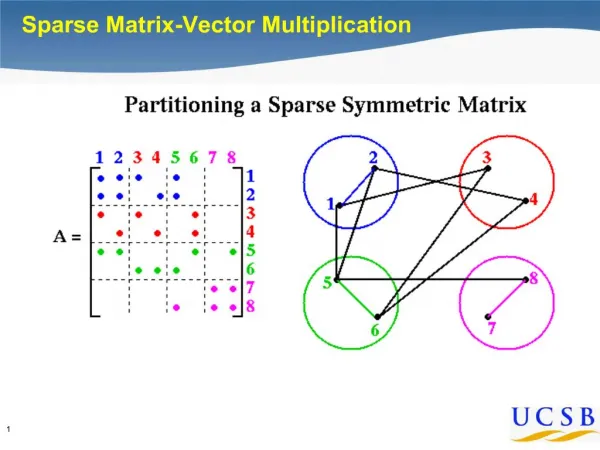
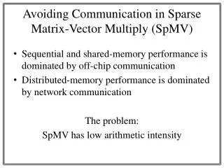
Avoiding Communication in Sparse Matrix-Vector Multiply ( SpMV )
Avoiding Communication in Sparse Matrix-Vector Multiply ( SpMV ). Sequential and shared-memory performance is dominated by off-chip communication Distributed-memory performance is dominated by network communication The problem: SpMV has low arithmetic intensity.

Avoiding Communication in Sparse Matrix-Vector Multiply ( SpMV )
E N D
Presentation Transcript
Avoiding Communication in Sparse Matrix-Vector Multiply (SpMV) • Sequential and shared-memory performance is dominated by off-chip communication • Distributed-memory performance is dominated by network communication The problem: SpMV has low arithmetic intensity
SpMV Arithmetic Intensity (1) dimension: n = 5 number of nonzeros: nnz = 3n-2 (tridiagonalA) Assumption: A is invertible ⇒ nonzero in every row ⇒ nnz ≥ n overcounts flops by up to n(diagonal A)
SpMV Arithmetic Intensity (2) O( lg(n) ) O( 1 ) O( n ) more flops per byte A r i t h m e t i c I n t e n s i t y SpMV, BLAS1,2 FFTs Stencils (PDEs) Dense Linear Algebra (BLAS3) Lattice Methods Particle Methods • Arithmetic intensity := Total flops / Total DRAM bytes • Upper bound: compulsory traffic • further diminished by conflict or capacity misses
256.0 128.0 64.0 32.0 16.0 8.0 4.0 2.0 1.0 0.5 1/8 1/4 1/2 1 2 4 8 16 SpMV Arithmetic Intensity (3) • In practice, A requires at least nnzwords: • indexing data, zero padding • depends on nonzero structure, eg, banded or dense blocks • depends on data structure, eg, • CSR/C, COO, SKY, DIA, JDS, ELL, DCS/C, … • blocked generalizations • depends on optimizations, eg, index compression or variable block splitting Opteron 2356 (Barcelona) peak double precision floating-point rate attainable gflop/s stream bandwidth How to do more flops per byte? Reuse data (x, y, A) across multiple SpMVs • 2 flops per word of data • 8 bytes per double • flop:byteratio ≤ ¼ • Can’t beat 1/16 of peak! actual flop:byteratio
Combining multiple SpMVs (1) kindependent SpMVs • (1) used in: • Block Krylov methods • Krylov methods for multiple systems (AX = B) (2) k dependent SpMVs • (2) used in: • s-step Krylov methods, • Communication-avoiding Krylov methods • …to compute kKrylov basis vectors (3) k dependent SpMVs, in-place variant Def. Krylov space (given A, x, s): • (3) used in: • multigridsmoothers, power method • Related to Streaming Matrix Powers optimization for CA-Krylov methods • What if we can amortize cost of reading A over kSpMVs ? • (k-fold reuse of A)
(1) k independent SpMVs(SpMM) • SpMMoptimization: • Compute row-by-row • Stream A only once =
(2) kdependent SpMVs(Akx) Naïve algorithm (no reuse): • Akx (Akx) optimization: • Must satisfy data dependencies while keeping working set in cache
(2) kdependent SpMVs(Akx) Akx algorithm(reuse nonzeros of A):
(3) kdependent SpMVs, in-place (Akx, last-vector-only) • Last-vector-only Akx optimization: • Reuses matrix and vector k times, instead of once. • Overwrites intermediates without memory traffic • Attains O(k) reuse, even when nnz < n • eg, A is a stencil (implicit values and structure)
256.0 128.0 64.0 32.0 16.0 8.0 4.0 2.0 1.0 0.5 1/8 1/4 1/2 1 2 4 8 16 Avoiding Serial Communication • Reduce compulsory misses by reusing data: • more efficient use of memory • decreased bandwidth cost (Akx, asymptotic) • Must also consider latency cost • How many cachelines? • depends on contiguous accesses • When k = 16 ⇒ compute-bound? • Fully utilize memory system • Avoid additional memory traffic like capacityand conflict misses • Fully utilize in-core parallelism • (Note: still assumes no indexing data) • In practice, complex performance tradeoffs. • Autotune to find best k Opteron 2356 (Barcelona) peak DP attainable gflop/s Stream Bandwidth ? actual flop:byteratio
On being memory bound • Assume that off-chip communication (cache to memory) is bottleneck, • eg, that we express sufficient ILP to hide hits in L3 • When your multicore performance is bound by memory operations, is it because of latency or bandwidth? • Latency-bound: expressed concurrency times the memory access rate does not fully utilize the memory bandwidth • Traversing a linkedlist, pointer-chasing benchmarks • Bandwidth-bound: expressed concurrency times the memory access rate exceeds the memory bandwidth • SpMV, stream benchmarks • Either way, manifests as pipeline stalls on loads/stores (suboptimal throughput) • Caches can improve memory bottlenecks – exploit them whenever possible • Avoid memory traffic when you have temporal or spatial locality • Increase memory traffic when cache line entries are unused (no locality) • Prefetcherscan allow you to express more concurrency • Hide memory traffic when your access pattern has sequential locality (clustered or regularly strided access patterns)
Distributed-memory parallel SpMV • Harder to make general statements about performance: • Many ways to partition x, y, and A to P processors • Communication, computation, and load-balance are partition-dependent • What fits in cache? (What is “cache”?!) • A parallel SpMV involves 1 or 2 rounds of messages • (Sparse) collective communication, costly synchronization • Latency-bound (hard to saturate network bandwidth) • Scatter entries of x and/or gather entries of y across network • kSpMVs cost O(k) rounds of messages • Can we do kSpMVs in one round of messages? • k independent vectors? SpMM generalizes • Distribute all source vectors in one round of messages • Avoid further synchronization • k dependent vectors? Akx generalizes • Distribute source vector plus additional ghost zone entries in one round of messages • Avoid further synchronization • Last-vector-only Akx ≈ standard Akx in parallel • No savings discarding intermediates
Distributed-memory parallel Akx Example: tridiagonal matrix, k = 3, n = 40, p = 4 Naïve algorithm: k messages per neighbor Akx optimization: 1 message per neighbor
Polynomial Basis for Akx • Today we considered the special case of the monomials: • Stability problems - tends to lose linear independence • Converges to principal eigenvector • Given A, x, k > 0, compute where pj(A) is a degree-j polynomial in A. • Choose p for stability.
Tuning space for Akx • DLP optimizations: • vectorization • ILP optimizations: • Software pipelining • Loop unrolling • Eliminate branches, inline functions • TLP optimizations: • Explicit SMT • Memory system optimizations: • NUMA-aware affinity • Software prefetching • TLB blocking • Memory traffic optimizations: • Streaming stores (cache bypass) • Array padding • Cache blocking • Index compression • Blocked sparse formats • Stanza encoding • Distributed memory optimizations: • Topology-aware sparse collectives • Hypergraph partitioning • Dynamic load balancing • Overlapped communication and computation • Algorithmic variants: • Compositions of distributed-memory parallel, shared memory parallel, sequential algorithms • Streaming or explicitly buffered workspace • Explicit or implicit cache blocks • Avoiding redundant computation/storage/traffic • Last-vector-only optimization • Remove low-rank components (blocking covers) • Different polynomial bases pj(A) • Other: • Preprocessing optimizations • Extended precision arithmetic • Scalable data structures (sparse representations) • Dynamic value and/or pattern updates
Krylov subspace methods (1) • Want to solve Ax = b (still assume A is invertible) • How accurately can you hope to compute x? • Depends on condition number of A and the accuracy of your inputs A and b • condition number with respect to matrix inversion • cond(A) – how much A distorts the unit sphere (in some norm) • 1/cond(A) – how close A is to a singular matrix • expect to lose log10(cond(A)) decimal digits relative to (relative) input accuracy • Idea: Make successive approximations, terminate when accuracy is sufficient • How good is an approximation x0 to x? • Error: e0 = x0 - x • If you know e0, then compute x = x0 - e0 (and you’re done.) • Finding e0 is as hard as finding x; assume you never have e0 • Residual: r0 = b – Ax0 • r0 = 0 ⇔ e0 = 0, but they do not necessarily vanish simultaneously • cond(A) small ⇒ (r0small ⇒ e0 small)
Krylov subspace methods (2) • Given approximation xold, refine by adding a correction xnew= xold + v • Pick v as the ‘best possible choice’ from search space V • Krylov subspace methods: V := • 2. Expand V by one dimension • 3. xold =xnew. Repeat. • Once dim(V) = dim(A) = n, xnew should be exact • Why Krylov subspaces? • Cheap to compute (via SpMV) • Search spaces V coincide with the residual spaces - • makes it cheaper to avoid repeating search directions • K(A,z) = K(c1A - c2I, c3z) ⇒ invariant under scaling, translation • Without loss, assume |λ(A)|≤ 1 • As s increases, Ks gets closer to the dominant eigenvectors of A • Intuitively, corrections v should target ‘largest-magnitude’ residual components
Convergence of Krylov methods • Convergence = process by which residual goes to zero • If A isn’t too poorly conditioned, error should be small. • Convergence only governed by the angles θm between spaces Km and AKm • How fast does sin(θm) go to zero? • Not eigenvalues! You can construct a unitary system that results in the same sequence of residuals r0, r1, … • If A is normal, λ(A) provides bounds on convergence. • Preconditioning • Transforming A with hopes of ‘improving’ λ(A) or cond(A)
Conjugate Gradient (CG) Method Given starting approximation x0 to Ax = b, let p0 := r0 := b - Ax0. For m = 0, 1, 2, … until convergence, do: • Vector iterates: • xm = candidate solution • rm = residual • pm = search direction Correct candidate solution along search direction Update residual according to new candidate solution Expand search space • Communication-bound: • 1 SpMV operation per iteration • 2 dot productsper iteration Reformulate to use Akx Do something about the dot products
Applying Akx to CG (1) • Ignore x, α, and β, for now • Unroll the CG loop s times (in your head) • Observe that: • ie, two Akx calls • This means we can represent rm+j and pm+jsymbolically as linear combinations: • And perform SpMV • operations symbolically: • (same holds for Rj-1) vectors of length n vectors of length 2j+1 CG loop: For m = 0,1,…, Do
Applying Akx to CG (2) 6. Now substitute coefficient vectors for vector iterates (eg, for r) SpMV performed symbolically by shifting coordinates: CG loop: For m = 0,1,…, Do
Blocking CG dot products 7. Let’s also compute the 2j+1-by-2j+1 Gram matrices: Now we can perform all dot products symbolically: CG loop: For m = 0,1,…, Do
CA-CG Given approximation x0 to Ax = b, let Take s steps of CG without communication For j = 0 to s - 1, Do { For m = 0, s, 2s, …, until convergence, Do { Expand Krylov basis, using SpMM and Akx optimizations: Represent the 2s+1 inner products of length n with a 2s+1-by-2s+1 Gram matrix Communication (sequential and parallel) } End For Recover vector iterates: Represent SpMV operation as a change of basis (here, a shift): Communication (sequential only) CG loop: For m = 0,1,…, Do } End For Represent vector iterates of length n with vectors of length 2s+1 and 2s+2:
CA-CG complexity (3) • Using Gram matrix and coefficient vectors have additional costs for CA-CG: • Dense work (besides dot products/Gram matrix) does not increase with s: • CG ≈ 6sn • CA-CG ≈ 3(2s+1)(2s+n) ≈ (6s+3)n • Sequential memory traffic decreases (factor of 4.5) • CG ≈ 6sn reads, 3sn writes • CA-CG ≈ (2s+1)nreads, 3n writes b = cacheline size, p = number of processors
CA-CG tuning • Performance optimizations: • 3-term recurrence CA-CG formulation: • Avoid the auxiliary vector p. • 2x decrease in Akx flops, bandwidth cost and serial latency cost (vectors only - A already optimal) • 25% decrease in Gram matrix flops, bandwidth cost, and serial latency cost • Roughly equivalent dense flops • Streaming Akx formulation: • Interleave Akx and Gram matrix construction, then interleave Akx and vector reconstruction • 2x increase in Akx flops • Factor of s decrease in Akx sequential bandwidth and latency costs (vectors only - A already optimal) • 2x increase in Akx parallel bandwidth, latency • Eliminate Gram matrix sequential bandwidth and latency costs • Eliminate dense bandwidth costs other than 3n writes • Decreases overall sequential bandwidth and latency by O(s), regardless of nnz. • Stability optimizations: • Use scaled/shifted 2-term recurrence for Akx: • Increase Akx flops by (2s+1)n • Increase dense flops by an O(s2) term • Use scaled/shifted 3-term recurrence for Akx: • Increase Akx flops by 4sn • Increase dense flops by an O(s2) term • Extended precision: • Constant factor cost increases • Restarting: • Constant factor increase in Akx cost • Preconditioning: • Structure-dependent costs • Rank-revealing, reorthogonalization, etc… • Can also interleave Akx and Gram matrix construction without the extra work - • decreases sequential bandwidth and latency by 33% rather than a factor of s