Chapter 1: Mathematical Models and Data Analysis

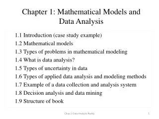
1. Chapter 1: Mathematical Models and Data Analysis 1.1 Introduction (case study example) 1.2 Mathematical models 1.3 Types of problems in mathematical modeling 1.4 What is data analysis? 1.5 Types of uncertainty in data 1.6 Types of applied data analysis and modeling methods 1.7 Example of a data collection and analysis system 1.8 Decision analysis and data mining 1.9 Structure of book Chap 1-Data Analysis-Reddy

2. Energy Use-Background • Energy use is central to the functioning and development of societies • Large amounts of energy are used in the world (and the United States in particular) • Even small annual increases in energy use has drastic results- exponential growth ( rates in developing countries are relatively large) • We are close to running out of conventional energy resources (currently supplies 85% of needs) • Energy use is causing other societal problems Chap 1-Data Analysis-Reddy

3. U.S. Primary Energy Consumption by Source and Sector, 2008(Quadrillion Btu) Source:  Energy Information Administration, Annual Energy Review 2008, Tables 1.3, 2.1b-2.1f , 10.3, and 10.4 Chap 1-Data Analysis-Reddy

4. U.S. Building Energy Scene • Buildings consume over 40% of the total energy • Also about 70% of electricity produced in US • Responsible for 49% SOx and 35% of CO2 • $785 billion (6.1% of GDP)- new construction • $483 billion (3.3% of GDP)- retrofits and repairs • 2003 CBECS study- over 85% of building stock build > 1990 About 2% undergo major retrofits each year • Opportunities in Commercial Building energy saving (OTA,1998): • Current cost-effective technology ~ $20 B/yr (25% energy savings) • - Advanced/Intelligent technology ~ $50 B/yr (over 50%) Chap 1-Data Analysis-Reddy

5. A typical building undergoes various phases during its life span in terms of its energy use: • Design phase (typical duration is 1-2 years) includes designing for energy efficiency • (i) conceptual or schematic design, where number of design alternatives • involving different types of feasible systems and their associated sub-systems (ii) detailed design and construction document preparation of the final design selected. (b) Construction (typical duration is 1-2 years) which includes: (i) civil construction (ii) installation of the various building systems, (iii) start-up commissioning to assure that various systems are installed properlyand are operating as intended. (c) Operation and maintenance (O&M) over its active life (typically 50-60 years for the shell, and 20-25 years for the MEP systems): (i) audits (ii) O&M assessment (iii) commissioning (iv) maintenance (v) condition monitoring, (vi) fault detection and diagnostics • (vii) active load control (viii) supervisory control (ix) monitoring and verification of energy conservation measures (d) Decommissioning Often 10 times more than the embodied or Initial energy Chap 1-Data Analysis-Reddy

6. Energy Conservation • In most cases energy conservation measures are more cost effective than supply side measures (such as renewables or new conventional power) • Over next 20 years, expected energy efficiency gains of: - 25-30% in most industrialized countries - over 40% in developing countries • MAJOR driver of sustainable development • Energy management allows one to better use existing power resources and defer new generation capacity Along with low energy design, important need to operate existing buildings efficiently- need for different skill sets Chap 1-Data Analysis-Reddy

7. Data analysis and modeling methods Used when performance data of the system is available for: • predicting the behavior of the system under different operating conditions, • identifying energy conservation opportunities, • verifying the effect of energy conservation measures and commissioning practices once implemented (M&V), • verifying that the system is performing as intended (called condition monitoring) • Operating the various sub-systems optimally (supervisory control) Chap 1-Data Analysis-Reddy

8. 1.2 Mathematical Models 1.2.1 One way of classifying data • Categorical (nominal, qualitative): non-numerical quality, ex. Male/female, pass/fail • Ordinal: has order or rank, ex. hot/mild/cold day • Count: number of items in certain classes • Metric: measurements of time, weight, height,… Dimensionality of data: univariate, bi-variate, multi-variate y=f(x1) y=f(x1, x2) Chap 1-Data Analysis-Reddy

9. Discrete and Continuous DataFig.1.1Fig. 1.2 Rolling of a dice (discrete data can only take on finite or countable number of values ) categorical, ordinal, count) (data can take on any continuous value, discretization is due to instrument) Chap 1-Data Analysis-Reddy

10. Source of data: • Population • Sample - single sample: single or successive readings taken at different times but under identical conditions - multi-sample: repeated measurements of same quantity by different instruments or observers • Two stage: staged experiments, second reading taken after first reading is analyzed Fig. 1.3 “Round-robin” experiment of testing the same solar thermal collector in six different test facilities (shown by different symbols) following the same testing methodology Chap 1-Data Analysis-Reddy

11. 1.2.2 What is a system model? A system is the object under study which could be as simple or as complex as one may wish to consider. It is any ordered, inter-related set of things, and their attributes. A model is a construct which allows one to represent the real-life system so that it can be used to predict the future behavior of the system under various “what-if” scenarios. Chap 1-Data Analysis-Reddy

12. 1.2.3 Types of Models (i) intuitive models(or qualitative or descriptive models) - non-analytical because only general qualitative trends of the system are known. Such a model which relies on quantitative or ordinal data is an aid to thought or to communication. Ex: Sociological or anthropological behavior (ii) empirical models-use metric or count data are those where the properties of the system can be summarized in a graph, a table or a curve fit to observation points. Such models presume some knowledge of the fundamental quantitative trends but lack accurate understanding. Econometric models are typical examples; and Chap 1-Data Analysis-Reddy

13. 1.2.3 Types of Models contd. (iii) mechanistic models(or structural models) which use metric or count data are based on mathematical relationships used to describe physical laws such as Newton’s laws, the laws of thermodynamics, etc... Such models can be used for prediction (system design) or for proper system operation and control (data analysis). Further such models can be separated into two sub-groups: • exact structural model where the model equation is thought to apply rigorously, • inexact structural models where the model equation applies only approximately, either because the process is not fully known or because one chose to simplify the exact model so as to make it more usable. Chap 1-Data Analysis-Reddy

14. System model f(x) A system model is a description of the system. Empirical and mechanistic models are made up of three components: (i) input variables(also referred to as regressor, forcing, exciting, exogenous or independent variables which act on the system: - controllable by the experimenter, - uncontrollable or extraneous such as climatic variables; (ii) system structure and parameters/properties provide the necessary physical description of the systems in terms of physical and material constants ; for example, thermal mass, overall heat transfer coefficients, mechanical properties of the elements; and (iii) output variables(also called response, state, endogenous or dependent variables) which describe system response to the input variables. Chap 1-Data Analysis-Reddy

15. Examples of Simple Models Pressure drop of fluid flowing through pipe Lumped model of water storage tank Can you identify the input variables, system parameters and output variables? Chap 1-Data Analysis-Reddy

16. Table 1.1 Ways of classifying mathematical models Chap 1-Data Analysis-Reddy

17. Fig. 1.4. Example of solid sphere cooling This system can be modeled as a lumped model provided the Biot number Bi <0.1. This number is proportional to the ratio of the heat conductive resistance (1/k) inside the sphere to the convective resistance (1/h) from the outer envelope of the sphere to the air. Chap 1-Data Analysis-Reddy

18. . Schematic 2R1C lumped model n th order lumped model • Figure 1.5 Thermal networks to model heat flow through a homogeneous plane wall of surface area A and wall thickness Chap 1-Data Analysis-Reddy

19. Linear vs Non-linear Figure 1.6 Principle of superposition of a linear system Chap 1-Data Analysis-Reddy

20. Linear vs Non-linear • An important distinction needs to be made between a linear model and a model which is linear in its parameters. For example, • is linear in both model and parameters a and b, • is a non-linear model but is linear in its parameters, and • is non-linear in both model and parameters. Chap 1-Data Analysis-Reddy

21. Simulation vs Performance Based Simulation models are used to predict system performance during the design phase when no actual system exists and alternatives are being evaluated. Performance based models rely on measured performance data of the actual system to provide insights into model structure and to estimate its parameters. • White-box models(also called detailed mechanistic models, reference models or small-time step models) are based on the laws of physics and permit accurate and microscopic modeling • Black-box models (or empirical or curve-fit or data-driven models) are based on little or no physical behavior of the system and rely on the available data to identify the model structure. • Gray-box modelsfall in-between the two above categories and are best suited for performance models Chap 1-Data Analysis-Reddy

22. Models for Sensor Response Steady-state models(also called zeroeth order models): - simplest model one can use. - They apply when input variables (and hence, the output variables) are maintained constant. A zeroeth order model for the dynamic performance of measuring systems is used (i) when the variation in the quantity to be measured is very slow as compared to how quickly the instrument responds, or (ii) as a standard of comparison for other more sophisticated models. For a zero-order instrument, the output is directly proportional to the input, such that (Doebelin, 1995): 1.7a 1.7b where a0 and b0 are the system parameters, assumed time invariant, qo and qi are the output and the input quantities respectively, K = b0 /a0 is called the static sensitivityof the instrument (only parameter needed to specify sensor response) Chap 1-Data Analysis-Reddy

23. The first-order model: or where is the time constantof the instrument = a1 / a0 , and K is the static sensitivity of the instrument which is identical to the value defined for the zeroeth model. Thus, two numerical parameters are used to completely specify a first-order instrument. 1.8b The solution to eq.1.8b for a step change in input is: 1.9 • where is the value of the input quantity after the step change. • The time constantcharacterizes the speed of response; the smaller its value the faster its response, and vice versa. • Numerically, the time constant represents the time taken for the response to reach 63.2% of its final change, or to reach a value within 36.8% of the final value. This is easily seen from eq. 1.9, by setting t= , in which case : Chap 1-Data Analysis-Reddy

24. Fig 1.2.7 Step-responses of two first-order instruments with different response times with assumed numerical values of time (x-axis) and instrument reading (y-axis). The response is characterized by the time constant which is the time for the instrument reading to reach 63.2% of the steady-state value Chap 1-Data Analysis-Reddy

25. Block Diagrams • Information flow or block diagramis a standard shorthand manner of schematically representing the inputs and output quantities of an element or a system as well as the computational sequence of variables. • Widely used during system simulation since a block implies that its output can be calculated provided the inputs are known. • They are very useful for setting up the set of model equations to solve in order to simulate or analyze systems or components. • Block diagrams should not be confused with material flow diagramswhich for a given system configuration are unique. On the other hand, there can be numerous ways of assembling block diagrams depending on how the problem is framed. Chap 1-Data Analysis-Reddy

26. Fig. 1.8 Schematic of a centrifugal pump rotating at speed s (say, in rpm) which pumps a water flow rate v from lower pressure p1 to higher pressure p2 Fig. 1.9 Different block diagrams for modeling a pump depending on how the problem is formulated Chap 1-Data Analysis-Reddy

27. 1.3 Types of Problems in Mathematical Modeling Consider the dynamic model of a component or system represented by the block diagram in Fig. 1.11. For simplicity, let us assume a linear model with no lagged terms in the forcing variables. Then, the model can be represented in matrix form as: Yt= AYt-1 + BUt + CWtwith Y1=d 1.10 where the output or state variable at time t is Yt. The forcing variables are of two types: -vector U denoting observable and controllable input variables, and -vector W indicating uncontrollable input variables or disturbing inputs. The parameter vectors of the model are {A, B, C} while d represents the initial condition vector. Fig. 1.11 Chap 1-Data Analysis-Reddy

28. Fig. 1.12 Different types of mathematical models used in forward and inverse approaches. The dotted line indicates that control problems often need model selection and parameter estimation as a first step. Chap 1-Data Analysis-Reddy

29. 1.3.2 Forward Problems Such problems are framed as one where: Given {U,W} and {B,C,d}, determine Y 1.11 The objective is to predict the response or state variables of a specified model with known structure and known parameters when subject to specified input or forcing variables (Fig.1.12). This is the type of models which is implicitly studied in classical mathematics and also in system simulation design courses. Unique solutions: Well-defined or well-specified problems: Degrees of freedom (df)=0 Chap 1-Data Analysis-Reddy

30. Solving the two equations simultaneously yields the performance conditions of the operating point, i.e., pressure drop and flow rate . Note that the numerical values of the model parameters are known, and that and V are the two variables, while the two equations provide the two constraints. Y B U Fig. 1.13 Example of a forward problem where solving two simultaneous equations, one representing the pump curve and the other the system curve, yields the operating point Chap 1-Data Analysis-Reddy

31. 1.3.3 Inverse Problems Generally speaking, inverse problems are those which involve identification of model structure and/or estimates of model parameters where the system under study already exists, and one uses measured or observed system behavior to aid in the model building. Different model forms may capture the data trend; this is why some argue that inverse problems are generally “ill-defined” or “ill-posed”. More than one possible solution, Degrees of freedom 0 Chap 1-Data Analysis-Reddy

32. Three types of inverse models all of which require some sort of identification or estimation (Fig. 1.12):  (a) calibrated forward models where ones uses a mechanistic model originally developed for the purpose of system simulation, and modifies or “tunes” the numerous model parameters so that model predictions match observed system behavior as closely as possible.   Given {Y”, U”, W”, d”}, determine {A”,B”,C”} 1.13awhere the “ notation is used to represent limited measurements or reduced parameter set; Over-constrained or under-parameterized problems: Degrees of freedom < 0 Chap 1-Data Analysis-Reddy

33. (b) model selection and parameter estimation where a suite of plausible model structures are formulated from basic scientific and engineering principles involving known influential and physically-relevant regressors, and performing experiments (or identifying system performance data) which allows these competing models to be evaluated and the “best” model identified Given {Y, U, W, d}, determine {A,B,C} 1.13b (c) models for system control and diagnostics Fig. 1.14 Example of a parameter estimation problem where the model parameters of a presumed function of pressure drop versus volume flow rate are identified from discrete experimental data points Statistical problems: Over-constrained or under-parameterized problems: Degrees of freedom > 0 Chap 1-Data Analysis-Reddy

34. Example 1.3.1 Simulation of a chiller Forward problem Fig. 1.15 Schematic of the cooling plant Chap 1-Data Analysis-Reddy

35. Five equations and five unknowns (d.f = 0): Cooling capacity: Chiller power 1st law balance HX in evaporator HX in condenser Solutions: Chap 1-Data Analysis-Reddy

36. Example 1.3.2: Dose-Response Curves Inverse problems The dots represent observed laboratory tests performed at high doses. Three types of models are fit to the data and all of them agree at high doses. However, they deviate substantially at low doses because the models are functionally different. - Model I is a nonlinear model applicable to highly toxic agents, - Model II is generally taken to apply to contaminants that are quite harmless as low doses (i.e., the body is able to metabolize the toxin at low doses). - Model III is an intermediate one between the other two curves. The above models are somewhat empirical (or black-box) and are useful as performance models. However, they provide little understanding of the basic process itself Fig. 1.16 Three different inverse models depending on toxin type for extrapolating dose-response observations at high doses to the response at low doses Chap 1-Data Analysis-Reddy

37. Issues relevant to inverse modeling (i) can the observed data of dose versus response provide some insights into the process which induces cancer in biological cells? • How valid are these results extrapolated down to low doses? • Since laboratory tests are performed on animal subjects, how valid are these results when extrapolated to humans? There are no simple answers to these queries (until the basic process itself is completely understood). The manner one chooses to extrapolate the dose-response curve downwards is dependent on either the assumption one makes regarding the basic process itself or how one chooses to err (which has policy-making implications). For example, erring conservatively in terms of risk would overstate the risk and prompt implementation of more precautionary measures, which some critics would fault as is improper use of limited resources. Chap 1-Data Analysis-Reddy

38. 1.4 What is Data Analysis? • “an evaluation of collected observations so as to extract information useful for a specific purpose” • “the process of systematically applying statistical and logical techniques to describe, summarize, and compare data”. Chap 1-Data Analysis-Reddy

39. Basic Steps in Statistical Data Analysis • Defining the problem The context of the problem and the exact definition of the problem being studied need to be defined. This allows one to design both the data collection system and the subsequent analysis procedures to be followed. • Collecting the data Nowadays the data is overwhelming, less care seems to be given to proper experimental design, different sources o data available, • Analyzing the data • Reporting the results Chap 1-Data Analysis-Reddy

40. 1.5 Types of Uncertainty in Data • purely stochastic variability (or aleatory uncertainty) where the ambiguity in outcome is inherent in the nature of the process, and no amount of additional measurements can reduce the inherent randomness. Examples involve coin tossing, or card games. These processes are inherently random (either on a temporal or spatial basis), and whose outcome, while uncertain, can be anticipated on a statistical basis; • epistemic uncertaintyor ignorance or lack of complete knowledge of the process which result in certain influential variables not being considered (and, thus, not measured); • inaccurate measurementof numerical data due to instrument or sampling errors; • cognitive vaguenessinvolving human linguistic description. For example, people use words like tall/short or very important/not important which cannot be quantified exactly. This type of uncertainty is generally associated with qualitative and ordinal data where subjective elements come into play. Chap 1-Data Analysis-Reddy

41. 1.6a Types of Methods (a) Exploratory data analysis and descriptive statistics, which entails performing “numerical detective work” on the data and developing methods for screening, organizing, summarizing and detecting basic trends in the data (such as graphs, and tables) which would help in information gathering and knowledge generation. (b) Model building and point estimation which involves (i) taking measurements of the various parameters (or regressor variables) affecting the output (or response variables) of a device or a phenomenon, (ii) identifying a causal quantitative correlation between them by regression, and (iii) using it to make predictions about system behavior under future operating conditions. (c) Inferential problems are those which involve making uncertainty inferences or calculating uncertainty or confidence intervals of population estimates from selected samples. They also apply to regression, i.e., uncertainty in model parameters, and in model predictions. Chap 1-Data Analysis-Reddy

42. 1.6b Types of Methods (d) Design of experiments is the process of prescribing the exact manner in which samples for testing need to be selected, and the conditions and sequence under which the testing needs to be performed such that the relationship or model between a response variable and a set of regressor variables can be identified in a robust and accurate manner. (e) Time series analysis and signal processing. Time series analysis involves the use of a set of tools that include traditional model building techniques as well as those involving the sequential behavior of the data and its noise. (f) Classification and clustering problems: Classification problems are those where one would like to develop a model to statistically distinguish or “discriminate” differences between two or more groups when one knows beforehand that such groupings exist in the data set provided, and, to subsequently assign, allocate or classify a future unclassified observation into a specific group with the smallest probability of error. Clustering, on the other hand, is a more difficult problem, involving situations when the number of clusters or groups is not known beforehand, and the intent is to allocate a set of observation sets into groups which are similar or “close” to one another with respect to certain attribute(s) or characteristic(s). Chap 1-Data Analysis-Reddy

43. 1.6c Types of Methods (f) Inverse modeling is an approach to data analysis methods which includes three classes: statistical calibration of mechanistic models, model selection and parameter estimation, and inferring forcing functions and boundary/initial conditions. It combines the basic physics of the process with statistical methods so as to get a better understanding of the system dynamics, and thereby use it to predict system performance either within or outside the temporal and/or spatial range used to develop the model. (h) Risk analysis and decision making: Analysis is often a precursor to decision-making in the real world. Along with engineering analysis there are other aspects such as making simplifying assumptions, extrapolations into the future, financial ambiguity,… that come into play while making decisions. Decision theory is the study of methods for arriving at “rational” decisions under uncertainty. The decisions themselves may or may not prove to be correct in the long term, but the process provides a structure for the overall methodology Chap 1-Data Analysis-Reddy

44. 1.7 Example of a data collection system Fig. 1.17 Flowchart depicting various stages in data analysis and decision making as applied to continuous monitoring of thermal systems Chap 1-Data Analysis-Reddy

45. 1.8 Decision analysis and data mining There are two disciplines with overlapping/complementary aims to that of data analysis and modeling. The first deals with decision analysis whose objective is to provide both an overall paradigm and a set of tools with which decision makers can construct and analyze a model of a decision situation. This is done after the data analysis phase The second discipline is data mining which is defined as the science of extracting useful information from large/enormous data sets. Though it is based on a range of techniques, from the very simple to the sophisticated (involving such methods as clustering techniques, artificial neural networks, genetic algorithms,…), it has the distinguishing feature that it is concerned with shifting through large/enormous amounts of data with no clear aim in mind except to discern hidden information, discover patterns and trends, or summarize data behavior Chap 1-Data Analysis-Reddy

46. Table 1.3 Analysis Methods Covered in Book Chap 1-Data Analysis-Reddy