Balanced Search Trees (Ch. 13)

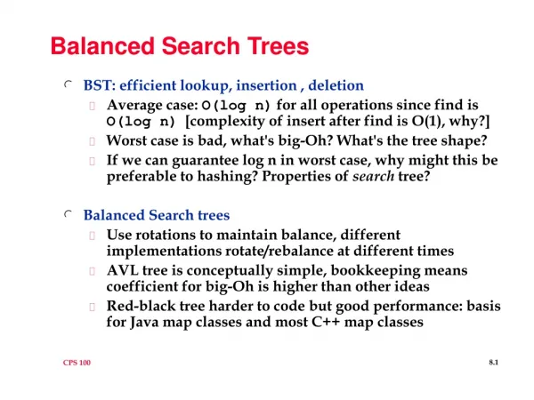
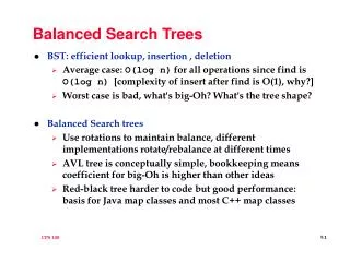
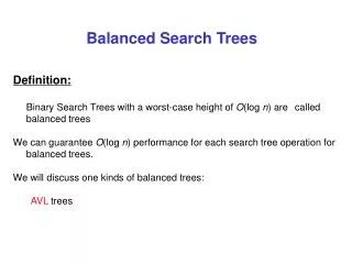
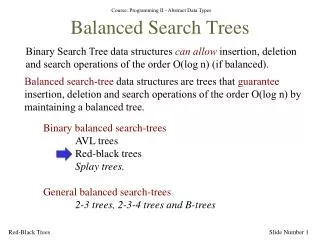
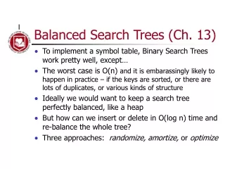
1. Balanced Search Trees (Ch. 13) • To implement a symbol table, Binary Search Trees work pretty well, except… • The worst case is O(n) and it is embarassingly likely to happen in practice – if the keys are sorted, or there are lots of duplicates, or various kinds of structure • Ideally we would want to keep a search tree perfectly balanced, like a heap • But how can we insert or delete in O(log n) time and re-balance the whole tree? • Three approaches: randomize, amortize, or optimize

2. Randomized BSTs • The randomized approach: introduce randomized decision making. • Dramatically reduce the chance of worst case. • Like quicksort, with random pivot • This algorithm is simple, efficient, broadly applicable – but went undiscovered for decades (until 1996!) [Only the analysis is complicated.] • Can you figure it out? How to introduce randomness in the created structure of the BST?

3. Random BSTs • Idea: to insert into a tree with n nodes, • with probability 1/(n+1) make the new node the root. • otherwise insert normally. • (this decision could be made at any point along the insertion path.) • result: about 2 n ln n comparisons to build tree; about 2 ln n for search • (that’s about 1.4 lg n)

4. How to insert at the root? • You might well ask: “that’s all well and good, but how do we insert at the root of a BST?” • I might well answer: Insert normally. Then rotate to move it up in the tree, until it is at the top. • Left and Right rotations: Rotate to the top!

5. Randomized BST analysis • The average case is the same for BSTs and RBSTs: but the essential point is that the analysis for RBSTs assumes nothing about the order of the insertions • The probability that the construction cost is more than k times the average is less than e-k • E.g. to build a randomized BST with 100,000 nodes, one would expect 2.3 million comparisons. The chance of 23 million comparisons is 0.01 percent. • Bottom line: • full symbol table ADT • straightforward implementation • O(log N) average case: bad cases provably unlikely

6. Splay Trees • Use root insertion • Idea: let’s rotate so as to better balance the tree • The difference between standard root insertion and splay insertion seem trivial: but the splay operation eliminates the quadratic worst case • The number of comparisons used for N splay insertions into an initially empty tree is O(N lg N) – actually, 3 N lg N. • amortized algorithm: individual operations may be slow, but the total runtime for a series of operations is good.

7. Splay Insertion • Orientations differ: same as root insertion • Orientations the same: do top rotation first • (brings nodes on search path closer to the root—how much?)

8. Splay Tree • When we insert, nodes on the search path are brought half way to the root. • This is also true if we splay while searching. • Trees at right are balanced with a few splay searches • left: smallest, next smallest, etc • right: random • Result: for M insert or search ops in an N-node splay tree, O((N+M)lg(N+M)) comparisons are required. • This is an amortized result.

9. 234 Intro • 234 Trees are are worst-case optimal: Q(log n) per operation • Idea: nodes have 1, 2, or 3 keys and 2, 3, or 4 links. • Subtrees have keys ordered analogously to a binary search tree. • A balanced 234 search tree has all leaves at the same level. • How would search work? • How would insertion work? • split nodes on the way back up? • or split 4-nodes on the way down?

10. Top-down vs. Bottom-up • Top-down 2-3-4 trees split nodes on the way down. But splitting a node means pushing a key back up, and it may have to be pushed all the way back up to the root. • It’s easier to split any 4-node on the way down. • 2-node with 4-node child: split into 3-node with two 2-node children • 3-node with 4-node child: split into 4-node with two 2-node children • Thus, all searches end up at a node with space for insertion

11. Construction Example

12. 234 Balance • All paths from the top to the bottom are the same height • What is that height? worst case: lgN (all 2-nodes) best case: lgN/2 (all 4-nodes) • height 10-20 for a million nodes; 15-30 for a billion • Optimal! • (But is it fast?)

13. Implementation Details • Actually, there are many 234-tree variants: • splitting on the way up vs. down • 2-3 vs. 2-3-4 trees • Implementation is complicated because of the large number of cases that have to be considered. • Can we improve the optimal balanced-tree approach, for fewer cases and strictly binary nodes?

14. B-trees • What about using even more keys? B-trees • Like a 234 tree, but with many keys, say b=100 or 500 • Usually enough keys to fill a 4k or 16k disk block • Time to find an item: O(logbn) • E.g. b=500: can locate an item in 500 with one disk access, 250,000 with 2, 125,000,000 with 3 • Used for database indexes, disk directory structures, etc., where the tree is too large for memory and each step is a disk access. • Drawback: wasted space

15. Red-Black Trees • Idea: Do something like a 2-3-4 Tree, but using binary nodes only The correspondence it not 1-1 because 3-nodes swing either way Add a bit per node to mark as Red or Black Black links bind together the 2-3-4 tree; red links bind the small binary trees holding 2, 3, or 4 nodes. (Red nodes are drawn with thick links to them.) Two red nodes in a row are not needed (or allowed)

16. Red-Black Tree Example • This tree is the same as the 2-3-4 tree built a few slides back, with the letters “ASEARCHINGEXAMPLE” • Notice that it is quite well balanced. (How well?) (We’ll see in a moment.)

17. RB-Tree Insertion • How do we search in a RB-tree? • How do we insert into a RB-tree? • normal BST insert; new node is red • How do we perform splits? • Two cases are easy: just change colors!

18. RB-Tree Insertion 2 • Two cases require rotations: Two adjacent red nodes – not allowed! If the 4-node is on an outside link, a single rotation is needed If the 4-node is on the center link, double rotation

19. RB-Tree Split • We can use the red-black abstraction directly • No two red nodes should be adjacent • If they become adjacent, rotatea red node up the tree • (In this case, a double rotationmakes I the root) • Repeat at the parent node • There are 4 cases • Details a bit messy: leave to STL!

20. Red-Black Tree Insertion link RBinsert(link h, Item item, int sw) { Key v = key(item); if (h == z) return NEW(item, z, z, 1, 1); if ((hl->red) && (hr->red)) { h->red = 1; hl->red = 0; hr->red = 0; } if (less(v, key(h->item))) { hl = RBinsert(hl, item, 0); if (h->red && hl->red && sw) h = rotR(h); if (hl->red && hll->red) { h = rotR(h); h->red = 0; hr->red = 1; } else { hr = RBinsert(hr, item, 1); if (h->red && hr->red && !sw) h = rotL(h); if (hr->red && hrr->red) { h = rotL(h); h->red = 0; hl->red = 1; } return h; } void STinsert(Item item) { head = RBinsert(head, item, 0); head->red = 0; }

21. RB Tree Construction

22. Red-Black Tree Summary • RB-Trees are BSTs with add’l properties: • Each node (or link to it) is marked either red or black • Two red nodes are never connected as parent and child • All paths from the root to a leaf have the same black-length • How close to being balanced are these trees? • According to black nodes: perfectly balanced • Red nodes add at most one extra link between black nodes • Height is therefore at most 2 log n.

23. Comparisons • There are several other balanced-tree schemes, e.g. AVL trees • Generally, these are BSTs, with some rotations thrown in to maintain balance • Let STL handle implementation details for you Build Tree Search Misses N BST RBST Splay RB Tree BST RBST Splay RB 5000 4 14 8 5 3 3 3 2 50000 63 220 117 74 48 60 46 36 200000 347 996 636 411 235 294 247 193

24. Summary • Goal: Symbol table implementation • O(log n) per operation • Randomized BST: O(log n) expected • Splay tree: O(log n) amortized • RB-Tree: O(log n) worst-case • The algorithms are variations on a theme: rotate during insertion or search to improve balance

25. STL Containers using RB trees • set: container for unique items • Member functions: insert() erase() find() count() lower_bound() upper_bound() iterators to move through the set in order • multiset: like set, but items can be repeated