9 Number Representation
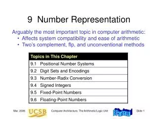
9 Number Representation. Arguably the most important topic in computer arithmetic: Affects system compatibility and ease of arithmetic Two’s complement, flp, and unconventional methods. 9.1 Positional Number Systems. Representations of natural numbers {0, 1, 2, 3, …}

9 Number Representation
E N D
Presentation Transcript
9 Number Representation • Arguably the most important topic in computer arithmetic: • Affects system compatibility and ease of arithmetic • Two’s complement, flp, and unconventional methods Computer Architecture, The Arithmetic/Logic Unit
9.1 Positional Number Systems • Representations of natural numbers {0, 1, 2, 3, …} • ||||| ||||| ||||| ||||| ||||| || sticks or unary code • 27 radix-10 or decimal code • 11011 radix-2 or binary code • XXVII Roman numerals • Fixed-radix positional representation with k digits • Value of a number: x = (xk–1xk–2 . . . x1x0)r = Sxi r i • For example: • 27 = (11011)two = (124) + (123) + (022) + (121) + (120) • Number of digits for [0, P]: k = logr (P + 1) = logr P + 1 k–1 i=0 Computer Architecture, The Arithmetic/Logic Unit
Unsigned Binary Integers Figure 9.1 Schematic representation of 4-bit code for integers in [0, 15]. Computer Architecture, The Arithmetic/Logic Unit
Representation Range and Overflow Figure 9.2 Overflow regions in finite number representation systems. For unsigned representations covered in this section, max – = 0. Example 9.2, Part d Discuss if overflow will occur when computing 317 – 316 in a number system with k = 8 digits in radix r = 10. Solution The result 86 093 442 is representable in the number system which has a range [0, 99 999 999]; however, if 317 is computed en route to the final result, overflow will occur. Computer Architecture, The Arithmetic/Logic Unit
9.2 Digit Sets and Encodings Conventional and unconventional digit sets Decimal digits in [0, 9]; 4-bit BCD, 8-bit ASCII Hexadecimal, or hex for short: digits 0-9 & a-f Conventional ternary digit set in [0, 2] Conventional digit set for radix r is [0, r – 1] Symmetric ternary digit set in [–1, 1] Conventional binary digit set in [0, 1] Redundant digit set [0, 2], encoded in 2 bits ( 0 2 1 1 0 )two and ( 1 0 1 0 2 )tworepresent 22 Computer Architecture, The Arithmetic/Logic Unit
The Notion of Carry-Save Addition Digit-set combination: {0, 1, 2} + {0, 1} = {0, 1, 2, 3} = {0, 2} + {0, 1} Figure 9.3 Adding a binary number or another carry-save number to a carry-save number . Computer Architecture, The Arithmetic/Logic Unit
9.3 Number Radix Conversion Two ways to convert numbers from an old radix r to a new radix R Perform arithmetic in the new radix R Suitable for conversion from radix r to radix 10 Horner’s rule: (xk–1xk–2 . . . x1x0)r = (…((0 + xk–1)r + xk–2)r + . . . + x1)r + x0 (1 0 1 1 0 1 0 1)two = 0 + 1 1 2 + 0 2 2 + 1 5 2 + 1 11 2 + 0 22 2 + 1 45 2 + 0 90 2 + 1 181 Perform arithmetic in the old radix r Suitable for conversion from radix 10 to radix R Divide the number by R, use the remainder as the LSD and the quotient to repeat the process 19 / 3 rem 1, quo 6 / 3 rem 0, quo 2 / 3 rem 2, quo 0 Thus, 19 = (2 0 1)three Computer Architecture, The Arithmetic/Logic Unit
Justifications for Radix Conversion Rules Justifying Horner’s rule. Figure 9.4 Justifying one step of the conversion of x to radix 2. Computer Architecture, The Arithmetic/Logic Unit
9.4 Signed Integers We dealt with representing the natural numbers Signed or directed whole numbers = integers { . . . , -3, -2, -1, 0, 1, 2, 3, . . . } Signed-magnitude representation +27 in 8-bit signed-magnitude binary code 0 0011011 –27 in 8-bit signed-magnitude binary code 1 0011011 –27 in 2-digit decimal code with BCD digits 1 0010 0111 Biased representation Represent the interval of numbers [-N, P] by the unsigned interval [0, P + N]; i.e., by adding N to every number Computer Architecture, The Arithmetic/Logic Unit
Two’s-Complement Representation With k bits, numbers in the range [–2k–1, 2k–1 – 1] represented. Negation is performed by inverting all bits and adding 1. Figure 9.5 Schematic representation of 4-bit 2’s-complement code for integers in [–8, +7]. Computer Architecture, The Arithmetic/Logic Unit
Conversion from 2’s-Complement to Decimal Example 9.7 Convert x = (1 0 1 1 0 1 0 1)2’s-compl to decimal. Solution Given that x is negative, one could change its sign and evaluate –x. Shortcut: Use Horner’s rule, but take the MSB as negative –1 2 + 0 –2 2 + 1 –3 2 + 1 –5 2 + 0 –10 2 + 1 –19 2 + 0 –38 2 + 1 –75 Sign Change for a 2’s-Complement Number Example 9.8 Given y = (1 0 1 1 0 1 0 1)2’s-compl, find the representation of –y. Solution –y = (0 1 0 0 1 0 1 0) + 1 = (0 1 0 0 1 0 1 1)2’s-compl (i.e., 75) Computer Architecture, The Arithmetic/Logic Unit
Two’s-Complement Addition and Subtraction Figure 9.6 Binary adder used as 2’s-complement adder/subtractor. Computer Architecture, The Arithmetic/Logic Unit
9.5 Fixed-Point Numbers Positional representation: k whole and l fractional digits Value of a number: x = (xk–1xk–2. . .x1x0.x–1x–2 . . . x–l )r = Sxi r i For example: 2.375 = (10.011)two = (121) + (020) + (02-1) + (12-2) + (12-3) Numbers in the range [0, rk – ulp] representable, where ulp = r–l Fixed-point arithmetic same as integer arithmetic (radix point implied, not explicit) Two’s complement properties (including sign change) hold here as well: (01.011)2’s-compl = (–021) + (120) + (02–1) + (12–2) + (12–3) = +1.375 (11.011)2’s-compl = (–121) + (120) + (02–1) + (12–2) + (12–3) = –0.625 Computer Architecture, The Arithmetic/Logic Unit
Fixed-Point 2’s-Complement Numbers Figure 9.7 Schematic representation of 4-bit 2’s-complement encoding for (1 + 3)-bit fixed-point numbers in the range [–1, +7/8]. Computer Architecture, The Arithmetic/Logic Unit
Radix Conversion for Fixed-Point Numbers Convert the whole and fractional parts separately. To convert the fractional part from an old radix r to a new radix R: Perform arithmetic in the new radix R Evaluate a polynomial in r–1: (.011)two = 0 2–1+ 1 2–2+ 1 2–3 Simpler: View the fractional part as integer, convert, divide by rl (.011)two = (?)ten Multiply by 8 to make the number an integer:(011)two = (3)ten Thus, (.011)two = (3 / 8)ten= (.375)ten Perform arithmetic in the old radix r Multiply the given fraction by R, use the whole part as the MSD and the fractional part to repeat the process (.72)ten = (?)two 0.72 2 = 1.44, so the answer begins with 0.1 0.44 2 = 0.88, so the answer begins with 0.10 Computer Architecture, The Arithmetic/Logic Unit
Significand Exponent Exponentbase 9.6 Floating-Point Numbers Useful for applications where very large and very small numbers are needed simultaneously Fixed-point representation must sacrifice precision for small values to represent large values x = (0000 0000 . 0000 1001)two Small number y = (1001 0000 . 0000 0000)two Large number Neither y2 nor y / x is representable in the format above Floating-point representation is like scientific notation: -20 000 000 = -2 1070.000 000 007 = 7 10–9 Also, 7E-9 Computer Architecture, The Arithmetic/Logic Unit
ANSI/IEEE Standard Floating-Point Format (IEEE 754) Revision (IEEE 754R) is being considered by a committee Short exponent range is –127 to 128 but the two extreme values are reserved for special operands (similarly for the long format) Figure 9.8 The two ANSI/IEEE standard floating-point formats. Computer Architecture, The Arithmetic/Logic Unit
Short and Long IEEE 754 Formats: Features Table 9.1 Some features of ANSI/IEEE standard floating-point formats Computer Architecture, The Arithmetic/Logic Unit
10 Adders and Simple ALUs • Addition is the most important arith operation in computers: • Even the simplest computers must have an adder • An adder, plus a little extra logic, forms a simple ALU Computer Architecture, The Arithmetic/Logic Unit
10.1 Simple Adders Digit-set interpretation: {0, 1} + {0, 1} = {0, 2} + {0, 1} Digit-set interpretation: {0, 1} + {0, 1} + {0, 1} = {0, 2} + {0, 1} Figures 10.1/10.2 Binary half-adder (HA) and full-adder (FA). Computer Architecture, The Arithmetic/Logic Unit
Full-Adder Implementations Figure10.3 Full adder implemented with two half-adders, by means of two 4-input multiplexers, and as two-level gate network. Computer Architecture, The Arithmetic/Logic Unit
Critical path Ripple-Carry Adder: Slow But Simple Figure 10.4 Ripple-carry binary adder with 32-bit inputs and output. Computer Architecture, The Arithmetic/Logic Unit
10.2 Carry Propagation Networks gi = xiyi pi = xiyi Figure 10.5 The main part of an adder is the carry network. The rest is just a set of gates to produce the g and p signals and the sum bits. Computer Architecture, The Arithmetic/Logic Unit
Ripple-Carry Adder Revisited The carry recurrence: ci+1 = gipici Latency of k-bit adder is roughly 2k gate delays: 1 gate delay for production of p and g signals, plus 2(k – 1) gate delays for carry propagation, plus 1 XOR gate delay for generation of the sum bits Figure 10.6 The carry propagation network of a ripple-carry adder. Computer Architecture, The Arithmetic/Logic Unit
The Complete Design of a Ripple-Carry Adder gi = xiyi pi = xiyi Figure 10.6 (ripple-carry network) superimposed on Figure 10.5 (general structure of an adder). Computer Architecture, The Arithmetic/Logic Unit
First Carry Speed-Up Method: Carry Skip Figures 10.7/10.8 A 4-bit section of a ripple-carry network with skip paths and the driving analogy. Computer Architecture, The Arithmetic/Logic Unit
10.3 Counting and Incrementation Figure 10.9 Schematic diagram of an initializable synchronous counter. Computer Architecture, The Arithmetic/Logic Unit
0 0 x1 x0 Figure 10.10 Carry propagation network and sum logic for an incrementer. Circuit for Incrementation by 1 Figure 10.6 Substantially simpler than an adder 1 Computer Architecture, The Arithmetic/Logic Unit
h j i i+1 10.4 Design of Fast Adders Carries can be computed directly without propagation For example, by unrolling the equation for c3, we get: c3 = g2p2c2 = g2p2g1p2p1g0p2p1p0c0 We define “generate” and “propagate” signals for a block extending from bit position a to bit position b as follows: g[a,b] = gbpbgb–1 pbpb–1gb–2 . . . pbpb–1…pa+1 ga p[a,b] = pbpb–1. . . pa+1 pa Combining g and p signals for adjacent blocks: g[h,j] = g[i+1,j]p[i+1,j]g[h,i] p[h,j] = p[i+1,j]p[h,i] [h, j] = [i + 1, j] ¢ [h, i] Computer Architecture, The Arithmetic/Logic Unit
Carries as Generate Signals for Blocks [0, i] Assuming c0 = 0, we have ci = g[0,i –1] Figure 10.5 Computer Architecture, The Arithmetic/Logic Unit
Second Carry Speed-Up Method: Carry Lookahead Figure 10.11 Brent-Kung lookahead carry network for an 8-digit adder, along with details of one of the carry operator blocks. Computer Architecture, The Arithmetic/Logic Unit
Recursive Structure of Brent-Kung Carry Network Figure 10.12 Brent-Kung lookahead carry network for an 8-digit adder, with only its top and bottom rows of carry-operators shown. Computer Architecture, The Arithmetic/Logic Unit
Carry-Lookahead Logic with 4-Bit Block Figure 10.13 Blocks needed in the design of carry-lookahead adders with four-way grouping of bits. Computer Architecture, The Arithmetic/Logic Unit
Third Carry Speed-Up Method: Carry Select Allows doubling of adder width with a single-mux additional delay Figure 10.14 Carry-select addition principle. Computer Architecture, The Arithmetic/Logic Unit
10.5 Logic and Shift Operations Conceptually, shifts can be implemented by multiplexing Figure 10.15 Multiplexer-based logical shifting unit. Computer Architecture, The Arithmetic/Logic Unit
Arithmetic Shifts Purpose: Multiplication and division by powers of 2 sra $t0,$s1,2 #$t0($s1) right-shifted by 2 srav $t0,$s1,$s0 #$t0($s1) right-shifted by ($s0) Figure 10.16 The two arithmetic shift instructions of MiniMIPS. Computer Architecture, The Arithmetic/Logic Unit
Practical Shifting in Multiple Stages Figure 10.17 Multistage shifting in a barrel shifter. Computer Architecture, The Arithmetic/Logic Unit
Bit Manipulation via Shifts and Logical Operations Bits 10-15 AND with mask to isolate a field: 0000 0000 0000 0000 1111 1100 0000 0000 Right-shift by 10 positions to move field to the right end of word The result word ranges from 0 to 63, depending on the field pattern Figure 10.18 A 4 8 block of a black-and-white image represented as a 32-bit word. Computer Architecture, The Arithmetic/Logic Unit
Logic unit 0 Arith unit 1 10.6 Multifunction ALUs Logic fn (AND, OR, . . .) Operand 1 Result Operand 2 Select fn type (logic or arith) Arith fn (add, sub, . . .) General structure of a simple arithmetic/logic unit. Computer Architecture, The Arithmetic/Logic Unit
An ALU for MiniMIPS Figure 10.19 A multifunction ALU with 8 control signals (2 for function class, 1 arithmetic, 3 shift, 2 logic) specifying the operation. Computer Architecture, The Arithmetic/Logic Unit