Normalization
Normalization. IS698 Min Song. Chapter Objectives. The purpose of normailization Data redundancy and Update Anomalies Functional Dependencies The Process of Normalization First Normal Form (1NF) Second Normal Form (2NF) Third Normal Form (3NF). Chapter Objectives (2).

Normalization
E N D
Presentation Transcript
Normalization IS698 Min Song
Chapter Objectives • The purpose of normailization • Data redundancy and Update Anomalies • Functional Dependencies • The Process of Normalization • First Normal Form (1NF) • Second Normal Form (2NF) • Third Normal Form (3NF)
Chapter Objectives (2) • General Definition of Second and Third Normal Form • Boyce-Codd Normal Form (BCNF)
The Purpose of Normalization Normalizationis a technique for producing a set of relations with desirable properties, given the data requirements of an enterprise. The process of normalization is a formal method that identifies relations based on their primary or candidate keys and the functional dependencies among their attributes.
Update Anomalies Relations that have redundant data may have problems called update anomalies, which are classified as , Insertion anomalies Deletion anomalies Modification anomalies
Example of Update Anomalies To insert a new staff with branchNo B007 into the StaffBranch relation; To delete a tuple that represents the last member of staff located at a branch B007; To change the address of branch B003. StaffBranch Figure 1 StraffBranch relation
Example of Update Anomalies (2) Staff Branch Figure 2 Straff and Branch relations
Functional Dependencies Functional dependency describes the relationship between attributes in a relation. For example, if A and B are attributes of relation R, and B is functionally dependent on A ( denoted A B), if each value of A is associated with exactly one value of B. ( A and B may each consist of one or more attributes.) B is functionally A B dependent on A Determinant Refers to the attribute or group of attributes on the left-hand side of the arrow of a functional dependency
Functional Dependencies (2) • FD is a way of representing relationship among attributes in a relation. • Notation • X Y where both X and Y can be a group of attributes. • We say that • X uniquely determines Y • For a given value of X, there is at most one value of Y associated with X at a time.
Functional Dependencies (3) Trival functional dependencymeans that the right-hand side is a subset ( not necessarily a proper subset) of the left- hand side. For example: staffNo, sName sName staffNo, sName staffNo They do not provide any additional information about possible integrity constraints on the values held by these attributes. We are normally more interested in nontrivial dependencies because they represent integrity constraints for the relation.
Functional Dependencies (3) Main characteristics of functional dependencies in normalization • Have a one-to-one relationship between attribute(s) on the left- and right- hand side of a dependency; • hold for all time; • are nontrivial.
The FD in a given relation are determined by the semantics of the relation not by data instances • TEACH looks to satisfy TEXT COURSE • Instance can be used to disprove a FD • TEACHER -\-> COURSE • COURSE -\-> TEXT • COURSE -\-> TEACHER
Exercise EMP_DEPT(ENAME, SSN, BDATE, DNUMBER, DNAME, DMGRSSN, DLOC) The FDs in this relation are: 1) SSN ENAME, BDATE, ADDRESS, DNUMBER 2) DNUMBER DNAME, DMGRSSN, DLOC Note: Each table much represent only one concept.
How to find meaningful FDs? • List only most direct FDs, not indirect FD. (e.g., SSN DLOC is an indirect FD) • List only meaningful FDs that we want to enforce as IC (e.g., SSN SSN is a trivial FD) • Do not include redundant attributes in an FD in either LHS or RHS
Functional Dependencies (4) Identifying the primary key Functional dependencyis a property of the meaning or semantics of the attributes in a relation. When a functional dependency is present, the dependency is specified as a constraint between the attributes. An important integrity constraint to consider first is the identification of candidate keys, one of which is selected to be the primary key for the relation using functional dependency.
Finding a key (Osburn’s algorithm) • Find attributes not appearing in the RHS of any FDs. Then, these are part of any candidate keys. • Check whether they can determine all other attributes by using FDs. • If not, what other attributes do I need to add to determine all other attributes?
Examples • STORE(SNAME, ADDR, ZIP, ITEM, PRICE) • FDs: SNAME ADDR ADDR ZIP SNAME, ITEM PRICE Finding a key: • SNAME does not appear in RHS, so SNAME must be a part of the key. • Since SNAME ADDR ZIP, we know SNAME ADDR, ZIP • But SNAME alone cannot determine any more. • How can we determine ITEM and PRICE? • If we have ITEM, them we can determine PRICE • So, SNAME, ITEM SNAME, ADDR, ZIP, ITEM, PRICE. So it satisfies the definition of the key
Lossless Decomposition • Decomposition means dividing a table into multiple tables • Decomposition is lossless (or nonloss) if it is possible to reconstruct R from decomposed relations using JOINs. • Condition for lossless join when R was decomposed into R1, R2, … Rn. • R = R1 R2 R3 …. Rn, where means JOIN operation. • Lossy decomposition • R R1 R2 R3 …. Rn
Why need it? • To maintain the accurate database • What if not? • Cause wrong answers for queries • How to check? • It is sufficient if any Ri contains a candidate key of R when we used the normalization algorithms for 3NF/BCNF. • This means that if any of the decomposed relation contains a complete CK (or PK) of the original relation, then the decomposition is called lossless. This means by joining all the decomposed relations, we can reconstruct the original relation.
Example 1 • LOAN_ACC(L#, AMT, ACC#, BAL) • L# AMT • ACC# BAL • Key? L# + ACC# • Possible decomposition: • R1(L#, AMT) R2(ACC#, BAL) • The decomposition is not loss-less since R1 and R2 do not have a candidate key.
Example 2 • WORK(EMP#, DEPT, LOC) • EMP# DEPT • DEPT LOC • Key? EMP# since EMP# DEPT, LOC • Decomposition: • R1(EMP#, DEPT) R2(DEPT, LOC) • The decomposition is loss-less since R1 contains a candidate key.
Functional Dependencies (5) • Armstrong’s axioms • Theorem: Armstrong’s axioms are sound and complete • Soundness: any result derived by applying the Armstrong’s axiom is always correct. • Completeness: Armstrong’s axiom can derive all the FDs that are necessary for computation of normalization. • We can fine all candidate keys by using Armstrong’s axiom. • We can compute the minimal cover of relations using Armstrong’s axiom.
Functional Dependencies (6) Inference Rules A set of all functional dependencies that are implied by a given set of functional dependencies X is called closure of X, written X+. A set of inference rule is needed to compute X+ from X. • Armstrong’s axioms • Relfexivity: If B is a subset of A, them A B • Augmentation: If A B, then A, C B • Transitivity: If A B and B C, then A C • Self-determination: A A • Decomposition: If A B,C then A B and A C • Union: If A B and A C, then A B,C • Composition: If A B and C D, then A,C B,
Functional Dependencies (6) Minial Sets of Functional Dependencies A set of functional dependencies X is minimal if it satisfies the following condition: • Every dependency in X has a single attribute on its • right-hand side • We cannot replace any dependency A B in X with • dependency C B, where C is a proper subset of A, and • still have a set of dependencies that is equivalent to X. • We cannot remove any dependency from X and still have a set of dependencies that is equivalent to X.
Functional Dependencies (7) Example of A Minial Sets of Functional Dependencies A set of functional dependencies for the StaffBranch relation satisfies the three conditions for producing a minimal set. staffNo sName staffNo position staffNo salary staffNo branchNo staffNo bAddress branchNo bAddress branchNo, position salary bAddress, position salary
The Process of Normalization • Normalization is often executed as a series of steps. Each step • corresponds to a specific normal form that has known properties. • As normalization proceeds, the relations become progressively • more restricted in format, and also less vulnerable to update • anomalies. • For the relational data model, it is important to recognize that • it is only first normal form (1NF) that is critical in creating • relations. All the subsequent normal forms are optional.
First Normal Form (1NF) Repeating group = (propertyNo, pAddress, rentStart, rentFinish, rent, ownerNo, oName) Unnormalized form (UNF) A table that contains one or more repeating groups. Figure 3 ClientRental unnormalized table
Definition of 1NF First Normal Form is a relation in which the intersection of each row and column contains one and only one value. * A relation R os om 1NF if all attributes have atomic values. • There are two approaches to removing repeating groups from • unnormalized tables: • Removes the repeating groups by entering appropriate data • in the empty columns of rows containing the repeating data. • 2. Removes the repeating group by placing the repeating data, • along with a copy of the original key attribute(s), in a separate • relation. A primary key is identified for the new relation.
1NF ClientRental relation with the first approach The ClientRental relation is defined as follows, ClientRental ( clientNo, propertyNo, cName, pAddress, rentStart, rentFinish, rent, ownerNo, oName) Figure 4 1NF ClientRental relation with the first approach With the first approach, we remove the repeating group (property rented details) by entering the appropriate client data into each row.
1NF ClientRental relation with the second approach Client (clientNo, cName) PropertyRentalOwner (clientNo, propertyNo, pAddress, rentStart, rentFinish, rent, ownerNo, oName) With the second approach, we remove the repeating group (property rented details) by placing the repeating data along with a copy of the original key attribute (clientNo) in a separte relation. Figure 5 1NF ClientRental relation with the second approach
Full functional dependency Full functional dependency indicates that if A and B are attributes of a relation, B is fully functionally dependent on A if B is functionally dependent on A, but not on any proper subset of A. A functional dependency AB is partially dependentif there is some attributes that can be removed from A and the dependency still holds.
Second Normal Form (2NF) Second normal form (2NF)is a relation that is in first normal form and every non-primary-key attribute is fully functionally dependent on the primary key. The normalization of 1NF relations to 2NF involves the removal of partial dependencies. If a partial dependency exists, we remove the function dependent attributes from the relation by placing them in a new relation along with a copy of their determinant.
Second Normal Form (2NF) Informal definition: A relation R is in 2NF if a) R is in 1NF and b) For each FD X A, X is not a part of any candidate key Condition b) means each attribute is fully functionally dependant on the whole key of R. The FD that does not satisfy the condition (b) is called a partial dependency (PD) Note: a non-Second Normal Form occurs only when you have a composite PK.
2NF ClientRental relation The ClientRental relation has the following functional dependencies: fd1 clientNo, propertyNo rentStart, rentFinish (Primary Key) fd2 clientNo cName (Partial dependency) fd3 propertyNo pAddress, rent, ownerNo, oName (Partial dependency) fd4 ownerNo oName (Transitive Dependency) fd5 clientNo, rentStart propertyNo, pAddress, rentFinish, rent, ownerNo, oName (Candidate key) fd6 propertyNo, rentStart clientNo, cName, rentFinish (Candidate key)
2NF ClientRental relation After removing the partial dependencies, the creation of the three new relations called Client, Rental, and PropertyOwner Client (clientNo, cName) Rental (clientNo, propertyNo, rentStart, rentFinish) PropertyOwner (propertyNo, pAddress, rent, ownerNo, oName) Client Rental PropertyOwner Figure 6 2NF ClientRental relation
Third Normal Form (3NF) Transitive dependency A condition where A, B, and C are attributes of a relation such that if A B and B C, then C is transitively dependent on A via B (provided that A is not functionally dependent on B or C). Third normal form (3NF) A relation that is in first and second normal form, and in which no non-primary-key attribute is transitively dependent on the primary key. The normalization of 2NF relations to 3NF involves the removal of transitive dependencies by placing the attribute(s) in a new relation along with a copy of the determinant.
Third Normal Form (3NF) Third normal form (3NF) Note that a TD exists between two non-key attributes. That is, if you have anyFD whose LHS is not a PK (CK), then R is not in 3NF. That is, each non-key attribute must be functionally dependent on the key and nothing else.
Example) • WORK(EMP#, ENAME, DEPT#, BUDGET, LOC) 2NF 3NF • EMP# ENAME Y Y • EMP# DEPT# Y Y • DEPT# BUDGET Y N • DEPT# LOC Y N WORK is in 2NF but not in 3NF because of FD (3) and (4)
3NF DECOMPOSITION algorithm • Combine the RHS of FDs if they have common LHS(union rule). • Create a separate table for each FD. • If there is any table, which is a subset of another, remove it. Ex: When you have R1(A,B,C,D) and R2(A,B), remove R2. • Check for lossless join If not lossless, then add a table consisting of a CK.
Example 1: 1) Combine the RHS of FDs if they have common LHS • EMP# ENAME, DEPT# • DEPT# BUDGET, LOC 2) Create a separate table for each FD R1(EMP#, ENAME, DEPT#), R2(DEPT#, BUDGET, LOC) 3) Check for redundant table 4) Check for lossless join The decomposition is lossless since R1 contains EMP# • The original relation WORK is not in 3NF but R1 and R2 are in 3NF. • Note that the LHS of a FD becomes the PK of each decomposed table.
Example 2: • LOAN_ACC(L#, AMT, LOAN_DATE, ACC#, BAL, ACC_DATE) • L# AMT • L# LOAN_DATE • ACC# BAL • ACC# ACC_DATE • Key L# + ACC# • Combine the RHS of FDs of they have common LHS. L# AMT, LOAN_DATE ACC# BAL, ACC_DATE 2) Create a separate table for each FD R1(L#, AMT, LOAN_DATE) R2(ACC#, BAL, ACC_DATE) 3) Check for redundant tables. 4) Check for lossless join The decomposition is lossy since neither R1 nor R2 contains L# + ACC#. So add the candidate key ad the 3rd relation. R3(L#,ACC#)
3NF ClientRental relation The functional dependencies for the Client, Rental and PropertyOwner relations are as follows: Client fd2 clientNo cName (Primary Key) Rental fd1 clientNo, propertyNo rentStart, rentFinish (Primary Key) fd5 clientNo, rentStart propertyNo, rentFinish (Candidate key) fd6 propertyNo, rentStart clientNo, rentFinish (Candidate key) PropertyOwner fd3 propertyNo pAddress, rent, ownerNo, oName(Primary Key) fd4 ownerNo oName (Transitive Dependency)
3NF ClientRental relation The resulting 3NF relations have the forms: Client (clientNo, cName) Rental (clientNo, propertyNo, rentStart, rentFinish) PropertyOwner (propertyNo, pAddress, rent, ownerNo) Owner (ownerNo, oName)
3NF ClientRental relation Rental Client PropertyOwner Owner Figure 7 2NF ClientRental relation
Boyce-Codd Normal Form (BCNF) Boyce-Codd normal form (BCNF) A relation is in BCNF, if and only if, every determinant is a candidate key. The difference between 3NF and BCNF is that for a functional dependency A B, 3NF allows this dependency in a relation if B is a primary-key attribute and A is not a candidate key, whereas BCNF insists that for this dependency to remain in a relation, A must be a candidate key.
Example of BCNF fd1 clientNo, interviewDate interviewTime, staffNo, roomNo (Primary Key) fd2 staffNo, interviewDate, interviewTime clientNo (Candidate key) fd3 roomNo, interviewDate, interviewTime clientNo, staffNo (Candidate key) fd4 staffNo, interviewDate roomNo (not a candidate key) As a consequece the ClientInterview relation may suffer from update anmalies. For example, two tuples have to be updated if the roomNo need be changed for staffNo SG5 on the 13-May-02. ClientInterview Figure 8 ClientInterview relation
Example of BCNF(2) To transform the ClientInterview relation to BCNF, we must remove the violating functional dependency by creating two new relations called Interview and SatffRoom as shown below, Interview (clientNo, interviewDate, interviewTime, staffNo) StaffRoom(staffNo, interviewDate, roomNo) Interview StaffRoom Figure 9 BCNF Interview and StaffRoom relations