Classical IPC Problems

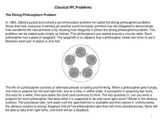
1. Classical IPC Problems The Dining Philosophers Problem In 1965, Dijkstra posed and solved a synchronization problem he called the dining philosophers problem. Since that time, everyone inventing yet another synchronization primitive has felt obligated to demonstrate how wonderful the new primitive is by showing how elegantly it solves the dining philosophers problem. The problem can be stated quite simply as follows. Five philosophers are seated around a circular table. Each philosopher has a plate of spaghetti. The spaghetti is so slippery that a philosopher needs two forks to eat it. Between each pair of plates is one fork. The life of a philosopher consists of alternate periods of eating and thinking. When a philosopher gets hungry, she tries to acquire her left and right fork, one at a time, in either order. If successful in acquiring two forks, she eats for a while, then puts down the forks and continues to think. The key question is: can you write a program for each philosopher that does what it is supposed to do and never gets stuck? Below is the obvious solution. The procedure take_fork waits until the specified fork is available and then seizes it. Unfortunately, the obvious solution is wrong. Suppose that all five philosophers take their left forks simultaneously. None will be able to take their right forks, and there will be a deadlock. 1

2. #define N 5 /* number of philosophers */ void philosopher(int i) /* i: philosopher number, from 0 to 4 */ { while (TRUE) { think(); /* philosopher is thinking */ take_fork(i); /* take left fork */ take_fork((i+1) % N); /* take right fork; % is modulo operator */ eat(); /* yum-yum, spaghetti */ put_fork(i); /* put left fork back on the table */ put_fork((i+1) % N); /* put right fork back on the table */ } } We could modify the program so that after taking the left fork, the program checks to see if the right fork is available. If it is not, the philosopher puts down the left one, waits for some time, and then repeats the whole process. This proposal too, fails, although for a different reason. With a little bit of bad luck, all the philosophers could start the algorithm simultaneously, picking up their left forks, seeing that their right forks were not available, putting down their left forks, waiting, picking up their left forks again simultaneously, and so on, forever. A situation like this, in which all the programs continue to run indefinitely but fail to make any progress is called starvation. (It is called starvation even when the problem does not occur in an Italian or a Chinese restaurant.)‏ #define N 5 /* number of philosophers */ #define LEFT (i+N-1)%N /* number of i's left neighbor */ #define RIGHT (i+1)%N /* number of i's right neighbor */ #define THINKING 0 /* philosopher is thinking */ #define HUNGRY 1 /* philosopher is trying to get forks */ #define EATING 2 /* philosopher is eating */ typedef int semaphore; /* semaphores are a special kind of int */ int state[N]; /* array to keep track of everyone's state */ semaphore mutex = 1; /* mutual exclusion for critical regions */ semaphore s[N]; /* one semaphore per philosopher */ 2

3. void philosopher(int i) /* i: philosopher number, from 0 to N1 */ { while (TRUE){ /* repeat forever */ think(); /* philosopher is thinking */ take_forks(i); /* acquire two forks or block */ eat(); /* yum-yum, spaghetti */ put_forks(i); /* put both forks back on table */ } } void take_forks(int i) /* i: philosopher number, from 0 to N1 */ { down(&mutex); /* enter critical region */ state[i] = HUNGRY; /* record fact that philosopher i is hungry */ test(i); /* try to acquire 2 forks */ up(&mutex); /* exit critical region */ down(&s[i]); /* block if forks were not acquired */ } void put_forks(i) /* i: philosopher number, from 0 to N1 */ { down(&mutex); /* enter critical region */ state[i] = THINKING; /* philosopher has finished eating */ test(LEFT); /* see if left neighbour can now eat */ test(RIGHT); /* see if right neighbour can now eat */ up(&mutex); /* exit critical region */ } void test(i) /* i: philosopher number, from 0 to N1* / { if (state[i] == HUNGRY && state[LEFT] != EATING && state[RIGHT] != EATING) { state[i] = EATING; up(&s[i]); } } 3

4. CPU Scheduling CPU scheduling is the basis of multiprogrammed operating systems. By switching the CPU among processes, the operating system can make the computer more productive. We will introduce basic CPU-scheduling concepts and present several CPU-scheduling algorithms. We also consider the problem of selecting an algorithm for a particular system. We have introduced threads to the process model. On operating systems that support them, it is kernel-level threads - not processes - that are in fact being scheduled by the operating system. However, the terms process scheduling and thread scheduling are often used interchangeably. In this chapter, we use process scheduling when discussing general scheduling concepts and thread scheduling to refer to thread-specific ideas. CHAPTER OBJECTIVES • To introduce CPU scheduling, which is the basis for multiprogrammed operating systems. • To describe various CPU-scheduling algorithms. • To discuss evaluation criteria for selecting a CPU-scheduling algorithm for a particular system. 4

5. Basic concepts In a single-processor system, only one process can run at a time; any others must wait until the CPU is free and cm be rescheduled. The objective of multiprogramming is to have some process running at all times, to maximize CPU utilization. The idea is relatively simple. A process is executed until it must wait, typically for the completion of some I/O request. In a simple computer system, the CPU then just sits idle. All this waiting time is wasted; no useful work is accomplished. With multiprogramming, we try to use this time productively. Several processes ,are kept in memory at one time. When one process has to wait, the operating system takes the CPU away from that process and gives the CPU to another process. This pattern continues. Every time one process has to wait, another process can take over use of the CPU. Scheduling of this kind is a fundamental opera ting system function. Almost all computer resources are scheduled before use. The CPU is, of course, one of the primary computer resources. Thus, its scheduling is central to operating-system design. 5

6. CPU-I/O Burst Cycle The success of CPU scheduling depends on an observed property of processes: Process execution consists of a cycle of CPU execution and I/O wait. Processes alternate between these two states. Process execution begins with a CPU burst. That is followed by an I/O burst, which is followed by another CPU burst, then another I/O burst, and so on. Eventually, the final CPU burst ends with a system request to terminate execution. The durations of CPU bursts have been measured extensively. Although they vary greatly from process to process and from computer to computer, they tend to have a frequency curve similar to that shown below. The curve is generally characterized as exponential or hyperexponential, with a large number of short CPU bursts and a small number of long CPU bursts. An l/O-bound program typically has many short CPU bursts. Whenever the CPU becomes idle, the operating system must select one of the processes in the ready queue to be executed. The selection process is carried out by the short-term scheduler (or CPU scheduler). The scheduler selects a process from the processes in memory that are ready to execute and allocates the CPU to that process. 6

7. Preemptive Scheduling CPU-scheduling decisions may take place under the following four circumstances: When a process switches from running state to the waiting state (for example, as the result of an I/O request or an invocation termination of one of the child processes). When a process switches from the running state to the ready state (for example, when an interrupt occurs). When a process switches from the waiting state to the ready state (for example, at completion of I/O). When a process terminates. For situations 1 and 4, there is no choice in terms of scheduling. A new process (if one exists in the ready queue) must be selected for execution. There is a choice, however, for situations 2 and 3. When scheduling takes place only under circumstances 1 and 4, we say that the scheduling scheme is nonpreemptive or cooperative; otherwise, it is preemptive. Under nonpreemptive scheduling, once the CPU has been allocated to a process, the process keeps the CPU until it releases it, either by terminating or by switching to the waiting state. This scheduling method was used by Microsoft Windows 3.x; Windows 95 introduced preemptive scheduling, and all subsequent versions of Windows operating systems have used preemptive scheduling. The Mac OSX operating system for the Macintosh uses preemptive scheduling; previous versions of the Macintosh operating system relied on cooperative scheduling. Cooperative scheduling is the only method that can be used on certain hardware platforms, because it does not require the special hardware (for example, a timer) needed for preemptive scheduling. 7

8. Preemption also affects the design of the operating-system kernel. During the processing of a system call, the kernel may be busy with an activity on behalf of a process. Such activities may involve changing important kernel data (for instance, I/O queues). What happens if the process is preempted in the middle of these changes and the kernel (or the device driver) needs to read or modify the same structure? Chaos ensues. Certain operating systems, including most versions of UNIX, deal with this problem by waiting either for a system call to complete or for an I/O block to take place before doing a context switch. This scheme ensures that the kernel structure is simple, since the kernel will not preempt a process while the kernel data structures are in an inconsistent state. Unfortunately, this kernel-execution model is a poor one for supporting real-time computing and multiprocessing. • Because interrupts can, by definition, occur at any time, and because they cannot always be ignored by the kernel, the sections of code affected by interrupts must be guarded from simultaneous use. The operating system needs to accept interrupts at almost all times; otherwise, input might be lost or output overwritten. So that these sections of code are not accessed concurrently by several processes, they disable interrupts at entry and reenable interrupts at exit. It is important to note that sections of code that disable interrupts do not occur very often and typically contain few instructions. • Dispatcher • Another component involved in the CPU-scheduling function is the dispatcher The dispatcher is the module that gives control of the CPU to the process selected by the short-term scheduler. This function involves the following: • Switching to text • Switching to user mode • The dispatcher should be as fast as possible, since it is invoked during every process switch. The time it takes for the dispatcher to stop one process and start another running is known as the dispatch latency. 8

9. Scheduling Criteria • Different CPU scheduling algorithms have different properties and the choice of a particular algorithm may favour one class of processes over another. In choosing which algorithm to use in a particular situation, we must consider the properties of the various algorithms. • Many criteria have been suggested for comparing CPU scheduling algorithms. Which characteristics are used for comparison can make a substantial difference in which algorithm is judged to be best. The criteria include the following: • CPU utilization. We want to keep the CPU as busy as possible. Conceptually, CPU utilization can range from 0 to 100 percent. In a real system, it should range from 40 percent (for a lightly loaded system) to 90 percent (for a heavily used system). • Throughput. If the CPU is busy executing processes, then work is being done. One measure of work is the number of processes that are completed per time unit, called throughput. For long processes, this rate may be one process per hour; for short transactions, it may be 10 processes per second. • Turnaround time. From the point of view of a particular process, the important criterion is how long it takes to execute that process. The interval from the time of submission of a process to the time of completion is the turnaround time. Turnaround time is the sum of the periods spent waiting to get into memory, waiting in the ready queue, executing on the CPU and doing I/O. • Waiting time. The CPU scheduling algorithm does not affect the amount of time during which a process executes or does I/O; it affects only the amount of time that a process spends waiting in the ready queue. Waiting time is the sum of periods spent waiting in the ready queue. • Response time. In an interactive system, turnaround time may not be the best criterion. Often, a process can produce some output fairly early and can continue computing new results while previous results are being output to the user. Thus, another measure is the time from the submission of a request until the first response is produced. This measure called response time, is the time it takes to start responding, not the time it takes to output the response. The turnaround time is generally limited by the speed of the output device. • It is desirable to maximize the CPU utilization and throughput and to minimize turnaround time, waiting time and response time. 9

10. Process Burst Time P1 24 P2 3 P3 3 Scheduling algorithms First-Come, First-Served Scheduling By far the simplest CPU-scheduling algorithm is the first-come, first-served (FCFS) scheduling algorithm. With this scheme, the process that requests the CPU first is allocated the CPU first. The implementation of the FCFS policy is easily managed with a FIFO queue. When a process enters the ready queue, its PCB (Process Control Block) is linked onto the tail of the queue. When the CPU is free, it is allocated to the process at the head of the queue. The running process is then removed from the queue. The code for FCFS scheduling is simple to write and understand. The average waiting time under the FCFS policy, however, is often quite long. Consider the following set of processes that arrive at time 0, with the length of the CPU burst given in milliseconds: If the processes arrive in the order P1, P2, P3, and are served in FCFS order, we get the result shown in the following Gantt chart: The waiting time is 0 milliseconds for process P1, 24 milliseconds for process P2, and 27 milliseconds for process P3. Thus, the average waiting time is (0 + 24 + 27)/3 = 17 milliseconds. If the processes arrive in the order P7, P3, Pi, however, the results will be as shown in the following Gantt chart: 10

11. The average waiting time is now (6 + 0 + 3)/3 = 3 milliseconds. This reduction is substantial. Thus, the average waiting time under an FCFS policy is generally not minimal and may vary substantially if the process's CPU burst times vary greatly. In addition, consider the performance of FCFS scheduling in a dynamic situation. Assume we have one CPU-bound process and many I/O-bound processes. As the processes flow around the system, the following scenario may result. The CPU-bound process will get and hold the CPU. During this time, all the other processes will finish their I/O and will move into the ready queue, waiting for the CPU. While the processes wait in the ready queue, the I/O devices are idle. Eventually, the CPU-bound process finishes its CPU burst and moves to an I/O device. All the I/O-bound processes, which have short CPU bursts, execute quickly and move back to the I/O queues. At this point, the CPU sits idle. The CPU-bound process will then move back to the ready queue and be allocated the CPU. Again, all the I/O processes end up waiting in the ready queue until the CPU-bound process is done. There is a convoy effect as all the other processes wait for the one big process to get off the CPU. This effect results in lower CPU and device utilization than might be possible if the shorter processes were allowed to go first. The FCFS scheduling algorithm is nonpreemptive. Once the CPU has been allocated to a process, that process keeps the CPU until it releases the CPU, either by terminating or by requesting I/O. The FCFS algorithm is thus particularly troublesome for time-sharing systems, where it is important that each user get a share of the CPU at regular intervals. It would be disastrous to allow one process to keep the CPU for an extended period. Shortest-Job-First Scheduling A different approach to CPU scheduling is the shortest-job-first (SJF) scheduling algorithm. This algorithm associates with each process the length of the process's next CPU burst. When the CPU is available, it is assigned to the process that has the smallest next CPU burst. If the next CPU bursts of two processes are the same, FCFS scheduling is used to break the tie. Note that a more appropriate term for this scheduling method would be the shortest-next-CPU-burst algorithm, because scheduling depends on the length of the next CPU burst of a process, rather than its total length. We use the term SJF because most people and textbooks use this term to refer to this type of scheduling. 11

12. Process Burst Time P1 6 P2 8 P3 7 P4 3 As an example of SJF scheduling, consider the following set of processes, with length of the CPU burst give in milliseconds: Using SJF scheduling, we would schedule these processes according to the following Gantt chart: The waiting time is 3 milliseconds for process P1, 16 milliseconds for process P2, 9 milliseconds for process P3, and 0 milliseconds for process P4. Thus, the average waiting time is (3 + 16 + 9 + 0)/4 = 7 milliseconds. By comparison, if we were using the FCFS scheduling scheme, the average waiting time would be 10.25 milliseconds. The SJF scheduling algorithm is provably optimal, in that it gives the minimum average waiting time for a given set of processes. Moving a short process before a long one decreases the waiting time of the short process more than it increases the waiting time of the long process. Consequently, the average waiting time decreases. The real difficulty with the SJF algorithm is knowing the length of the next CPU request. For long-term (job) scheduling in a batch system, we can use as the length the process time limit that a user specifies when he submits the job. Thus, users are motivated to estimate the process time limit accurately, since a lower value may mean faster response (Too low a value will cause a time-limit-exceeded error and require resubmission.). SJF scheduling is used frequently in long-term scheduling. 12

13. Although the SJF algorithm is optimal, it cannot be implemented at the level of short-term CPU scheduling. There is no way to know the length of the next CPU burst. One approach is to try to approximate SJF scheduling. We may not know the length of the next CPU burst, but we may be able to predict its value. We expect that the next CPU burst will be similar in length to the previous ones. Thus, by computing an approximation of the length of the next CPU burst, we can pick the process with the shortest predicted CPU burst. The next CPU burst is generally predicted as an exponential average of the measured lengths of previous CPU bursts. Let tn be the length of the nth CPU burst, and let τn+1 be our predicted value for the next CPU burst. Then, for α where This formula defines an exponential average. The value of tn contains our most recent information; τn stores the past history. The parameter α controls the relative weight of recent and past history in our prediction. If α=0, then tn+1 = τn and recent history has no effect (current conditions are assumed to be transient); if α=0, then τn+1 = tn, and only the most recent CPU burst matters (history is assumed to be old and irrelevant). More commonly, α = 1/2, so recent history and past history are equally weighted. The initial τ0 can be defined as a constant or as an overall system average. Figure below shows an exponential average with α=1/2 and τ0 =10. To understand the behaviour of the exponential average, we can expand the formula for τn+1 by substituting for τn to find Since both α and (1 - α) are less than or equal to 1, each successive term has less weight than its predecessor. The SJF algorithm can be either preemptive or nonpreemptive. The choice arises when a new process arrives at the ready queue while a previous process is still executing. The next CPU burst of the newly arrived process may be shorter than what is left of the currently executing process. A preemptive SJF algorithm will preempt the currently executing process, whereas a nonpreemptive SJF algorithm will allow the currently running process to finish its CPU burst. Preemptive SJF scheduling is sometimes called Shortest Remaining Time First Scheduling. 13

14. Process Arrival Time Burst Time P1 0 8 P2 1 4 P3 2 9 P4 3 5 As an example, consider the following four processes, with the length of the CPU burst given in milliseconds: 14

15. If the processes arrive at the ready queue at the times shown and. need the indicated burst times, then the resulting preemptive SJF schedule is as depicted in the following Gantt chart: Process P1 is started at time 0, since it is the only process in the queue. Process P2 arrives at time 1. The remaining time for process P1 (7 milliseconds) is larger than the time required by process P2 (4 milliseconds), so process P1 is preempted, and process P2 is scheduled. The average waiting time for this example is ((10-1) + (1-1) + (17-2) + (5-3))/4 = 26/4 = 6.5 milliseconds. Nonpreemptive SJF scheduling would result in an average waiting time of 7.75 milliseconds. Priority Scheduling The SJF algorithm is a special case of the general priority scheduling algorithm. A priority is associated with each process, and the CPU is allocated to the process with the highest priority. Equal-priority processes are scheduled in FCFS order. An SJF algorithm is simply a priority algorithm where the priority (p) is the inverse of the (predicted) next CPU burst. The larger the CPU burst, the lower the priority, and vice versa. Note that we discuss scheduling in terms of high priority and low priority. Priorities are generally indicated by some fixed range of numbers, such as 0 to 7 or 0 to 4,095. However, there is no general agreement on whether 0 is the highest or lowest priority. Some systems use low numbers to represent low priority; others use low numbers for high priority. This difference can lead to confusion. In this text, we assume that low numbers represent high priority. As an example, consider the following set of processes, assumed to have arrived at time 0, in the order P1, P2, • • •, P5, with the length of the CPU burst given in milliseconds: 15

16. Process Burst Time Priority P1 10 3 P2 1 1 P3 2 4 P4 1 5 P5 5 2 Using priority scheduling, we would schedule these processes according to the following Gantt chart: The average waiting time is 8.2 milliseconds. Priorities can be defined either internally or externally. Internally defined priorities use some measurable quantity or quantities to compute the priority of a process. For example, time limits, memory requirements, the number of open files, and the ratio of average I/O burst to average CPU burst have been used in computing priorities. External priorities are set by criteria outside the operating system, such as the importance of the process, the type and amount of funds being paid for computer use, the department sponsoring the work, and other, often political, factors. Priority scheduling can be either pre-emptive or nonpreemptive. When a process arrives at the ready queue, its priority is compared with the priority of the currently running process. A preemptive priority scheduling algorithm will pre-empt the CPU if the priority of the newly arrived process is higher than the priority of the currently running process. A nonpreemptive priority scheduling algorithm will simply put the new process at the head of the ready queue. A major problem with priority scheduling algorithms is indefinite blocking, or starvation. A process that is ready to run but waiting for the CPU can be considered blocked. A priority scheduling algorithm can leave some low-priority processes waiting indefinitely. In a heavily loaded computer system, a steady stream of higher-priority processes can prevent a low-priority process from ever getting the CPU. 16

17. Process Burst Time P1 24 P2 3 P3 3 Round-Robin Scheduling The round-robin (RR) scheduling algorithm is designed especially for time-sharing systems. It is similar to FCFS scheduling, but pre-emption is added to switch between processes. A small unit of time, called a time quantum or time slice, is defined. A time quantum is generally from 10 to 100 milliseconds. The ready queue is treated as a circular queue. The CPU scheduler goes around the ready queue, allocating the CPU to each process for a time interval of up to 1 time quantum. To implement RR scheduling, we keep the ready queue as a FIFO queue of processes. New processes are added to the tail of the ready queue. The CPU scheduler picks the first process from the ready queue, sets a timer to interrupt after 1 time quantum, and dispatches the process. One of two things will then happen. The process may have a CPU burst of less than 1 time quantum. In this case, the process itself will release the CPU voluntarily. The scheduler will then proceed to the next process in the ready queue. Otherwise, if the CPU burst of the currently running process is longer than 1 time quantum, the timer will go off and will cause an interrupt to the operating system. A context switch will be executed, and the process will be put at the tail of the ready queue. The CPU scheduler will then select the next process in the ready queue. The average waiting time under the RR policy is often long. Consider the following set of processes that arrive at time 0, with the length of the CPU burst given in milliseconds: If we use a time quantum of 4 milliseconds, then process P1 gets the first 4 milliseconds. Since it requires another 20 milliseconds, it is preempted after the first time quantum, and the CPU is given to the next process in the queue, process P2. Since process P2 does not need 4 milliseconds, it quits before its time quantum expires. The CPU is then given to the next process, process P3. Once each process has received 1 time quantum, the CPU is returned to process P1 for an additional time quantum. 17

18. The resulting RR schedule is The average waiting time is 17/3 = 5.66 milliseconds. In the RR scheduling algorithm, no process is allocated the CPU for more than 1 time quantum in a row (unless it is the only runnable process). If a process's CPU burst exceeds 1 time quantum, that process is preempted and is put back in the ready queue. The RR scheduling algorithm is thus preemptive. If there are n processes in the ready queue and the time quantum is q, then each process gets 1/n of the CPU time in chunks of at most q time units. Each process must wait no longer than (n-1) x q time units until its next time quantum. For example, with five processes and a time quantum of 20 milliseconds, each process will get up to 20 milliseconds every 100 milliseconds. The performance of the RR algorithm depends heavily on the size of the time quantum. At one extreme, if the time quantum is extremely large, the RR policy is the same as the FCFS policy. If the time quantum is extremely small (say, 1 millisecond), the RR approach is called processor sharing and (in theory) creates the appearance that each of n processes has its own processor running at 1/n the speed of the real processor. This approach was used in Control Data Corporation (CDC) hardware to implement ten peripheral processors with only one set of hardware and ten sets of registers. The hardware executes one instruction for one set of registers, then goes on to the next. This cycle continues, resulting in ten slow processors rather than one fast one. (Actually, since the processor was much faster than memory and each instruction referenced memory, the processors were not much slower than ten real processors would have been.)‏ 18