Download
1 / 102
1.04k likes | 1.23k Vues
Outline The infinite square well A comment on wavefunctions at boundaries Parity How to solve the Schroedinger Equation in momentum space Please read Goswami Chapter 6. The infinite square well Suppose that the sides of the finite square well are extended to infinity:

E N D
Outline • The infinite square well • A comment on wavefunctions at boundaries • Parity • How to solve the Schroedinger Equation in momentum space • Please read Goswami Chapter 6.
The infinite square well • Suppose that the sides of the finite square well are extended to infinity: • It is a simplified case of the finite square well. How they differ: • Finite case Infinite case • Since V is not infinite in Regions 1 and 3, Since V is infinite in Regions 1 and III, • it is possible to have small damped ψ there. no ψ can exist there. ψ must terminate • abruptly at the boundaries.
Finite case Infinite case To find the ψ’s use the boundary The abrupt termination of the wavefunction is conditions. nonphysical, but it is called for by this (also nonphysical) well. Abrupt change: we cannot require dψ/dx to be continuous at boundaries. Instead, replace the boundary conditions with: Solve for ψ in Region 2 only. Begin with ψ = Acoskx + Bsinkx Result: but require ψ = 0 at x = ± a/2. Result:
Comment on wavefunctions at boundaries • Anytime a wave approaches a change in potential, the wave has some probability of reflecting, regardless of whether its E is >V or <V. So consider: • Case 1: • Case 2: • Case 3: The wave will have some probability to reflect in all 3 cases. You cannot assume there is no “Be-ikx” in Region 1 of Cases 2 and 3. The way to see this is to work an example: Put in Aeikx + Be-ikx for Region 1 and see that the boundary conditions cannot be satisfied unless B ≠ 0. We will have a homework about this.
Linear combinations of wavefunctions • Suppose that somehow a particle in a well gets into this state: • u(x)=A sin 4πx/L + B sin 6πx/L • Questions: (1) What is its Ψ(x,t)? • (2) Is this a stationary state? • Answers: (1) Recall Ψ=u(x)T(t). Here u=u1 + u2, where each ui goes with a different energy state Ei of the infinite square well:
Parity • Parity is a property of a wavefunction.
What determines the parity of ψ ? The form of the potential V. The ψ’s that are eigenfunctions of some Hamiltonian H have definite parity (even or odd) if V(x)=V(-x). Prove this here:
So if ψ(x) is an eigenfunction of H, then so is ψ(-x). But we said ψ(x) is non-degenerate, so ψ(-x) cannot be independent of ψ(x).
IV. How to solve the Schroedinger Equation in momentum space: using p-space wavefunctions. Message: The Schroedinger Equation, and the states of matter represented by wavefunctions, are so general that theey exist outside of any particular representation (x or p) and can be treated by either. Example: Consider a potential shaped as V(x) = Cx for x > 0 = 0 for x ≤ 0
How to find the allowed energies in momentum space? Recall that any potential well produces quantized energies. We find them by applying boundary conditions (BC’s). Usually we have the BC’s expressed in x-space. So we must either convert BC’s to p-space or Convert A(p) to x-space. We will do this.
Outline • What to remember from linear algebra • Eigenvalue equations • Hamiltonian operators • The connection between physics and math in Quantum Mechanics • Please re-read Goswami Section 3.3. • Please read the Formalism Supplement.
Outline • Hilbert space • The linear algebra – Quantum Mechanics connection, continued • Dirac Notation
Outline • The Projection Operator • Position and momentum representations • Ways to understand the symbol <Φ|ψ> • Commutators and simultaneous measurements • Please read Goswami Chapter 7.
This is a vector. This is a scalar. So they can appear in any order. Now reorder them:
β c Φi
Position representation and momentum representation • Recall that the wavefunctions exist in abstract Hilbert space. To calculate with them, we must represent them in coordinate space or momentum space. • The goal of this section: to show that “representing ψ in a space” (for example, position space) means projecting it onto each of the basis vectors of that space. • To do this we will need 2 things: Hilbert ψ space p-space x-space