Insights into Data Mining Techniques and Regression Analysis
Explanation of multiple regression, data mining, attribute evaluation, and practical examples of regression in database management systems. Discover how to calculate information gain and analyze non-linear estimation methods.

Insights into Data Mining Techniques and Regression Analysis
E N D
Presentation Transcript
Database Management Systems:Data Mining Attribute Evaluation
Multiple Regression Y = b0 + b1X1 + b2X2 + … + bkXk Regression estimates the b coefficients. If a b value is zero, the corresponding X attribute does not influence the Y variable. The b value coefficient also indicates the strength of the relationship: dY/dXi = bi. A one unit increase in Xi results in a bi change in Y.
Regression Example: RT Query: Sales by Year by City Population: SELECT Format([orderdate],"yyyy") AS SaleYear, City.Population1990, Sum(Bicycle.SalePrice) AS SumOfSalePrice FROM City RIGHT JOIN (Customer INNER JOIN Bicycle ON Customer.CustomerID = Bicycle.CustomerID) ON City.CityID = Customer.CityID GROUP BY Format([orderdate],"yyyy"), City.Population1990 HAVING (((City.Population1990)>0)); Paste data into Exel. Tools/Data Analysis/Regression
Regression Results 75% variation explained Each year, sales increase $356 Less than 0.05, so significantly different from zero For 1000 people, sales increase $33
Information Gain: Partitioning In 1948, Shannon defined information (I) as: If pi is zero or one, there is no information—since you always know what will happen.
Information Example Types of shoppers (m=2): status is high roller or tourist S is a set of data (rows) The dataset contains attributes (A), such as: Income, Age_range, Region, and Gender. Each attribute has many (v) possible values. For example, Income categories are: low, medium, high, and wealthy. The subset Sij contains the rows of customers in category i who possess attribute level j. The count of the number of rows is sij. The entropy of attribute A defined from this partitioning is The information gain from the partitioning is Find the attribute with the highest gain.
Data for Information Example s1=104 s2=107 s=211 E(income)=0.2015 Gain(income) = 0.9999-0.2015 = 0.7984 =79/211*I(…)
Results for Information All values are relatively high, so all attributes are important.
Dimensionality • Notice the issue of dimensionality in the example. • We had to setup groups within the attributes. • If there are too many groupings/values: • The system will take a long time to run. • Many subgroups will have no observations. • How do you establish the groupings/values? • Natural hierarchies (e.g., dates) • Cluster analysis • Prior knowledge • Level of detail required for analysis
Non-Linear Estimation • Regression: • Polynomial: Y = b0 + b1X + b2X2 + b3X3 + b4X4…+ u • Exponential: Y = b0Xb1eu ln(Y) = ln(b0) + b1 ln(X) + u • Log-Linear: ln(Y) = b0 + b1 ln(X) + u • Other: log log and more • Other Methods: • Neural networks • Search
Example: PolyAnalyst: Find Law for MPG mpg = (2.59183e+009 *power*age+176465 *power*age*weight+2.41554e+009 *power*age*age-3.54349e+009 *power+7.27281e+007 *age*weight-2.55635e+010)/(power*age*weight+52028.3 *power*age*age*weight) Best exact rule found: mpg = (4.71047e+008 *power*age*weight-38783.5 *power*age*weight*weight+2.5987e+009 *power*age*age*weight-7.65205e+009 *power*weight+1.5658e+008 *age*weight*weight+1.15859e+011 *power*power-3.0532e+013 *age*age)/(power*age*weight*weight+52028.3 *power*age*age*weight*weight)
Problems with Non-Linear Models • They can be harder to estimate. • They are substantially more difficult to optimize. • They are often unstable—particularly at the ends. Y = 15000 – 850 X – 435 X2 + 2 X3 + X4 Note: (x + 7)(x – 5)(x + 20)(x – 20)