Simulation and Animation
Simulation and Animation. Fractals. Fractals and fractal landscapes. Fractals : „Die fraktale Geometrie der Natur“, B. Mandelbrot, Birkhäuser „The Science of Fractal Images“, H.-O. Peitgen , D.Saupe , Springer Verlag Fractal landscapes :


Simulation and Animation
E N D
Presentation Transcript
Simulation and Animation Fractals
Fractals and fractal landscapes Fractals: • „Die fraktale Geometrie der Natur“, B. Mandelbrot, Birkhäuser • „The Science ofFractal Images“, H.-O. Peitgen, D.Saupe, Springer Verlag Fractallandscapes: • „Texturing and Modeling, A Procedural Approach“ , D. Ebert et al. AP Professional, Cambridge – available in ourlibrary • www.wizardnet.com/musgrave/ • www.javaworld.com/javaworld/jw-08-1998/jw-08-step.html
Fractals and fractal landscapes Fractalshapes in nature:
Midpoint Displacement • Random MidpointDisplacement • Interpolation anddisplacement • Decreasingrandomdisplacements in eachiteration
Midpoint Displacement • Random displacements Di (i: subdivisionlevel) • Dihas normal distribution E[Di]=0 • Di = N(0,i2) = iN(0,1) • Standard deviation i • Variance(Di) = i2 =(i-1 1/2H)2 Xi+1(t) and 1/2H Xi(2t) arestatisticallyself-similar
Midpoint Displacement • Terrain generation • Interpolatenewvaluesfromadjacentvalues • Add randomdisplacement • Values areinfluencedbyadjacentsquares • Creasesareintroducedbyearlyiterations New points Old points
Midpoint Displacement • Terrain generation – the Diamond Square algorithm http://62.65.146.182/java/fractal/fract.htm http://users.bestweb.net/~hogdog/fractal.htm
Midpoint Displacement Successiverefinements in 2D
Fractals • Whatis a fractal • Well, many different fractalsexist
Fractals • Fractal = abbreviationfor „Fractional Dimension“ • Anycurveorsurfacethatisindependentofscale–itlooksthe same over all rangesofscale • Ifblownup in scale, anypartappearsidenticaltothewhole • „Exact“ Self-Similarity (DeterministicFractals) • Iterationsof a scalingprocess Sierpinski-Triangle Koch-Curve
Fractals Fractals • „Statistical“ Self-Similarity (StochasticFractals) • Ifblownup in scale, anypartappearsstatisticallysimilartothewhole
Fractals • Fractionaldimension • Measureforthe„roughness“of a curve/surface • E.g. a roughcurvemay cover thesurfaceitisdefined on • Somewherebetweendimension N and N+1 • Characterizestheincreaseofmeasuredlengthbetweengivenpointsasscaledecreases • L: numberofself-similarpieces • s: lengthofthepieces (in units)
Fractals • Fractional dimension • Example: The Koch-Curve • It fills more space than a line (D=1) but less space than a Euclidean area of the plane (D=2)
Fractal generation processes • Pick a startingpoint (x0,y0). • Choose an indexiwitha givenprobabilityp • Computethenextpointasfollows: xn+1= aixn+ biyn+ eiyn+1= cixn+ diyn+ fi • Plot thenewpointandgotostep 2 i a b c d e f p 0 0.00.0 0.0 0.16 0.0 0.0 0.10 1 0.2 -0.26 0.23 0.22 0.0 1.6 0.08 2 -0.15 0.28 0.26 0.24 0.0 0.44 0.08 3 0.750.04 -0.04 0.85 0.0 1.60 0.74
Fractal generation processes • IteratedFunction Systems • Repeatedtransformationof simple patterns on smallerandsmallerscales (bymeansof affine transformations) • Select transformation (fromsetofpossibletransformations) randomlywithcertainprobablity Example: Fern i a b c d e f p 0 0.0 0.0 0.0 0.16 0.0 0.0 0.10 1 0.2 -0.26 0.23 0.22 0.0 1.6 0.08 2 -0.15 0.28 0.26 0.24 0.0 0.44 0.08 3 0.75 0.04 -0.04 0.85 0.0 1.60 0.74
Fractal generation processes • Mandelbrot Set • Evaluaterecursivelyforinitalpoints c in complex plane • Color points in the plane correspondingto rate ofdivergence
Fractal generation processes • Julia Sets • Forfixed c, pointszion thecomplexplane forwhichdoesnot tendtoinfinity • Ormoregeneral: • zn+1 = f(zn) • E.g.: zn+1 = c sin(zn) zn+1 = c exp(zn)
Fractal generation processes StochasticFractals
Fractal generation processes • Stochastic Fractals • Simulation of Fractal Brownian motion (FBm) • Probability as a tool for modelling • Modelling of (dynamic) natural phenomena • Terrains, clouds, water etc. • Modelling and rendering of solid textures • Marble, wood etc. • Procedural shaders
Stochastic fractals • Brownian Motion • Discovered 1827 by botanist R. Brown • Behavior of pollen in water • Describes the movement of small particles of solid matter in liquid • Mathematical examination by Einstein and Wiener • Dynamics of molecular collisions • Pollen particles being hit by water molecules • Used by Mandelbrot for the modelling of natural phenomena
Stochasticfractals • Brownian Motion - a littlestatistics • Continuousrandom variable X • Probabilitydistributionfunction F(x) = P(Xx) • Probabilitydensityfunction f(x) 0 • Expectation E[X]: • VarianceVar[X] = E[(X-E[X])2]
Stochasticfractals • Brownianmotion – a littlestatistics • Example: Gaussian Distribution N(,2)
Stochasticfractals • Brownianmotion – „Random Walk Process“ • Brownianmotionis a stochastic (random) process • Describesthemovementof a particleover time t X(t+t) = X(t) + v · t · N(0,1) • X: particleposition • v: speedofparticle • N(0,1): normal distributedrandom variable
Stochastic fractals • Brownianmotion – properties • The increments X(t2)-X(t1) haveGaussiandistribution E[X(t2) – X(t1)] = 0 • Var[X(t2) – X(t1)] |t2-t1| • Continuous but nowheredifferentiable • Increments X(t+h)-X(t) areindependentof t • Brownianmotionisstationary
Stochastic fractals • Brownianmotion • IfX(t0)=0 X(t) and X(rt)/r0.5arestatisticallyequivalent • Brownianmotion – morethannoise!
Stochastic fractals • White noise (1/f0-noise) • Completelyuncorrelatedfrom sample to sample • Independent ofthepast • Flat spectrum – all frequencieswiththe same amountofenergy • Simulatedbythepseudo-randomgenerator
Stochastic fractals • 1/f-noise • Itiscorrelatedfrom sample to sample • Lowerfrequenciescontributemost • Oftenfound in nature (clouds, water, growthprocesses) • E.g. Kolmogorovsspectrum • Complexgenerationprocess • See nextchapter
Stochastic fractals • Brownianmotion • Itistheintegrationofwhitenoise – also called 1/f2-noise • More correlatedthanwhitenoiseand 1/f-noise • Correlated (constraint) random walk
Stochastic fractals • FractalBrownianmotion (FBm) • Extension ofBrownianmotion • Var[X(t2) – X(t1)] |t2-t1|2H • H: Hurst exponent • X(t), 1/rH X(rt) arestatisticallyself-similarwithrespectto H • 0 H 1 determinestheroughnessofthestructure
Stochasticfractals • FractalBrownianmotion (FBm) H = 0.5: incrementsare not correlated • Brownianmotion H > 0.5: incrementshave positive correlation • Increasingly smoother curves H < 0.5: incrementshave negative correlation Increasinglyroughercurves
Stochastic fractals • FractalBrownianmotion - 1/f-noise • Fractaldimension D = d+1-H = d + (3-)/2 • d: topologicaldimension • Curves: d=1: D = 2-H =(5-)/2 • Surfaces: d=2: D = 3-H =(7-)/2 • Volumes: d=3: D = 4-H =(9-)/2
Stochastic fractals • FBm = 1 D = 2 = 1.5 D = 1.75 = 2 (Bm) D = 1.5 = 2.5 D = 1.25 = 3 D = 1
Stochastic fractals • Generation processes for (multi-dimensional) FBm • Midpoint displacement • „Sum of sawtooth waves of successively doubled and scaled frequencies“ • Rescale-and-Add • „Sum of band-limited random basis functions with scaled frequencies“ • Fourier domain synthesis • „Sum of sine-waves with random phase and scaled frequencies“ Citations from K. Musgraves PhD thesis
Rescale-and-Add • Noise synthesis by point evaluation • Summation of scaled and dilated noise functions
Rescale-and-Add Add weighted noiseoctaves to simulate 1/f-noise weights 1/20 1/21 1/22 1/23 1/24 1/25 =
Rescale-and-Add Another method to simulate 1/f-noise Generate noisy copies on-the-fly from a base random field 1/24 1/23 1/22 = • • • 1/21 1/20
Rescale-and-Add • Noise synthesisbypointevaluation • Summation ofscaledanddilatednoisefunctions • S: noisefunction • N(0,1) distributedrandomnumbersgiven on „integer lattice“ • Band-limited, smooth, continuous • r: lacunarity: averagesizeofgaps (typically r=2) • Addingnoiseoctavesatdecreasingfrequency but increasingamplitude
Rescale-and-Add • Implementation of the Noise() function • Lattice noise • N(0,1) variables at grid points (lattice noise) • Multi-dimensional interpolation (value noise) • bi/tri-linearly • Spline-interpolation • Gradient noise • Compute pseudorandom gradients at grid points • Uniformly distributed over the unit circle (sphere in 3D) • For point p and each adjacent grid point compute • fraction = p – int[p] • gradient[int[p]] · fraction (is a scalar product) • Linearly interpolate results at p • Interpolation weights are 1- fraction
Gradient Noise • Given an input point • For each of its neighboring grid points: • Pick a "pseudo-random" gradient vector • Compute linear function (dot product) • Take weighted sum, using thease curves + + + =
Rescale-and-Add • Implementation of Noise() function • Memory optimization • Storing values at each grid point too expensive • Use hash table or permutation array • PermTab[N] = 5,1,28,43,11,... // permutation of first N-1 integers • NoiseTab[N] = 0.1, 0.7, ... // N N(0,1) random values • 2D example: Noise((int)x, (int)y) = NoiseTab[PermTab[(x+PermTab[y]) % N]]
Rescale-and-Add • Localparametervariation • Fractaldimension D = d+1-H • Anisotropicfractaldimension in spaceandtime • Oftencalledmultifractals (heterogeneousfractals)
Application of noise • Random surface texture • Color = white * noise(point)
Application of noise • Colored noise • Color = Colormap (noise(k*point)) • k controls the feature size - the larger k is, the smaller the feature
Application of noise • Classical Turbulence function(note similarity to Rescale-and-Add method) function turbulence(p) t = 0 scale = 1 while (scale > pixelsize) t += abs(Noise(p/scale)*scale) scale /= 2 return t
Application of noise Simulating marble effects function marble(p) x = p[1] + rurbulence(p) return marble_color(sin(x))
Application of noise Using turbulence to modulate sphere radius
Fourier Domain Synthesis • Fourier transform • Two different approachestodescribe a function • Spatialdomain vs. frequencydomain • Every reasonablefunction f canberepresentedas a superpositionofharmonic (sin/cos) functions • Output is an imaginarynumber S(t)=R(t)+iI(t)=S(t)ei(t) • S(t) : amplitude • (t) : phaseangle
Fourier Domain Synthesis • Fourier transform • Superposition of harmonic functions
Fourier Domain Synthesis • The discrete Fourier transform of images • The sampled Fourier transform contains frequencies needed to represent the domain