Wind-Driven Flow in a Lake: Hydrodynamic Equations and Pressure Friction Assumptions
170 likes | 261 Vues
Explore the governing equations and assumptions for wind-driven flow in a lake, including pressure-friction assumptions and hydrostatic pressure considerations. Discover how pressure gradients affect velocity profiles and stress distribution in turbulent flows.

Wind-Driven Flow in a Lake: Hydrodynamic Equations and Pressure Friction Assumptions
E N D
Presentation Transcript
CEE 262A HYDRODYNAMICS Lecture 13 Wind-driven flow in a lake
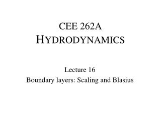
Wind-Driven Flow in a Lake Assumption (i) Steady Forcing (ii) Two-dimensional (iii) H/L<<1 (A turbulent stress) “Rigid lid” x3=H H x3=0 L x1=0 x1=L
The governing equations with hydrostatic pressures removed are: Mass: x1-Momentum: x3-Momentum: Simplify Effective viscosity – assumed constant (a) (b) Scale
~ ~ ~ To find U and P we use an assumed force balance: pressure ~ friction The free surface condition gives Since we are looking to make We find that
Mass: If we choose x1-Mom: From prev. slide: since which reduces to:
Likewise the x3-momentum eqn. becomes To end up with PC flow we must require two things: 2 If these conditions are both satisfied and we get rid of all of the small stuff, what is left is: Hydrostatic Pressure-friction
Assumption 1: H/L << 1 "The Long Box" H L Assumption 2: Horizontal advection time scale Vertical diffusion time scale << << Horizontal acceleration Vertical friction
The second equation implies that p* = p*(x1*). However, since the boundary conditions are independent of x1*, u1* should only be a function of x3*. This implies that the pressure gradient must be constant, i.e. not a function of x1*. Thus, we are back to the PC equations we solved before. But, how do we find ? We obtain an extra condition on u1* If we integrate continuity from x3*=0 to x3* = 1, we find that The pressure gradient we need is the one that imposes no net flow
So to proceed, we now use three conditions to constrain the quadratic velocity profile that results from integration of the x1 momentum equation No slip on bottom Specified stress on top No net flow l=2a=3/2
Thus putting it all together, we find that So that the velocity we find at the top is (to compare to our PC soln.) Since P = 3 (no net flow for PC flow), we can now compute the dimensional pressure gradient using our computed surface velocity and the definition:
Why the 3/2 ? Look at stress distribution and balance of forces Shear stress 1 Pressure -1/2 Net force per unit length = +3/2t0 = Pressure force/unit length = lH Note: For turbulent flows it has been found that the stress on the bottom is nearly zero, so that the 3/2 should really be 1 for real flows
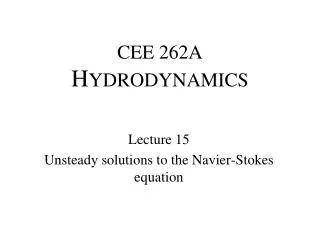
What happens when we blow a 7 m/s wind over a 2 km long channel that is 10 m deep? t0/r0=ra CD U102/r0=1.0 kg/m3 * 0.002 * 49 m2/s2/r0=10-4 m2/s2 ne~0.005 m2/s H2/ne = 334 min H = 10 m L = 2 km model (SUNTANS) No stress No slip
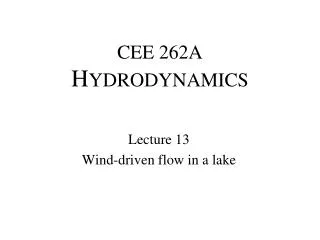
What provides the pressure gradient ? In nature, a sloping free surface From hydrostatics: Condition required so that domain is still rectangular and that x1 gradients are small where Water depth without applied stress Super elevation relative to x3=H x3=0 x1=L x1=0
Now if we compute the horizontal pressure gradient, we can solve for the surface slope This enables us to now integrate to find the water surface change due to winds.
Since generally all of the water that starts in the lake stays there If we integrate the slope equation wrt x1 Thus, the maximum change up or down is
zoomed-in view Previous example: Predicted HF oscillation: T = 2L/c0 = 2L/(gH)1/2 =6.7 min (time it takes for a shallow water wave to propagate from one end to the other and back) Computed: 0.001 m Less bottom stress!
Relative to the depth this change is: Normal example Lake Okeechobee during a hurricane