Lecture 2. Randomness
Lecture 2. Randomness. Goal of this lecture: We wish to associate incompressibility with randomness. But we must justify this. We all have our own “standards” (or tests) to decide if a sequence is random. Some of us have better tests.

Lecture 2. Randomness
E N D
Presentation Transcript
Lecture 2. Randomness • Goal of this lecture: We wish to associate incompressibility with randomness. • But we must justify this. • We all have our own “standards” (or tests) to decide if a sequence is random. Some of us have better tests. • In statistics, there are many randomness tests. If incompressible sequences pass all such effective tests, then we can happily call such sequences random sequences. • But how do we do it? Shall we list all randomness tests and prove our claim one by one?
Compression • A file (string) x, containing regularities that can be exploited by a compressor, can be compressed. • Compressor PPMZ finds more than bzip2, and bzip2 finds more than gzip, so PPMZ compresses better that bzip2, and bzip2 better than gzip. • C(x) is the ultimate in using every effective regularity in x: the shortest compressed version of x that can be decompressed by a single decompressor that works for every x. Hence at least as short as any (known or unknown) compressor can do.
Randomness • Randomness of strings mean that they do not contain regularities. • If the regularities are not effective, then we cannot use them. • Hence, we consider randomness of strings as the lack of effective regularities (that can be exploited). • For example: a random string cannot be compressed by any known or unknown real-world compressor.
Randomness, continued. • C(x) is the shortest program that can generate x, exploiting all effective regularity in x. • Example 1. Flipping a fair coin n times gives x that with high probability 99.9% that C(x)≥n-10. No real world compressor can compress such an x below n-10. • Example 2. The initial n bits of π=3.1415... cannot be compressed by any real-world compressor, because they don’t see the regularity. But there is a short program that generates π, so C(π|n)=O(1).
Intuition:Randomness = incompressibility • But we need a formal proof. So we formalize the notion of a single effective regularity. Such a regularity can be exploited by a Turing machine in the form of a test. • Then we formalize the notion of all possible effective regularities together, as those that can be exploited by the single Universal Turing Machine in the form of a universal test. • Strings x passing the universal test turn out to be the incompressible ones.
Preliminaries • We will write x=x1x2 … xn …, and xm:n =xm … xn and we usually deal with binary finite strings or binary infinite sequences. • For finite string x, we can simply define x to be random if C(x)≥|x| or C(x) ≥ |x| - c for small constant c. • But this does not work for infinite sequences x. For example if we define: x is random if for some c>0, for all n C(x1:n) ≥ n-c Then no infinite sequence is random. Proof of this fact: For an infinite x and an integer m>0, take n such that x1x2 … xm is binary representation of n-m. Then C(x1x2 .. xmxm+1 …xn) ≤ C(xm+1 … xn) + O(1) ≤ n-logn QED • We need a reasonable theory connecting incompressibility with randomness a la statistics. A beautiful theory is provided by P. Martin-Lof during 1964-1965 when he visited Kolmogorov in Moscow.
Martin-Lof’s theory • Can we identify “incompressibility” with “randomness” (as known from statistics)? • We all have our own “statistical tests”. Examples: • A random sequence must have ½ 0’s and ½ 1’s. Furthermore, ¼ 00’s, 01’s, 10’s 11’s. • A random sequence of length n cannot have a large (say length √n) block of 0’s. • A random sequence cannot have every other digit identical to corresponding digits of π. • We can list millions of such tests. • These tests are necessary but not sufficient conditions. But we wish our random sequence to pass all such (un)known tests! • Given sample space S and distribution P, we wish to test the hypothesis: “x is a typical outcome” --- that is: x belongs to some concept of “majority”. Thus a randomness test is to pick out the atypical minority y’s (e.g. too many more 1’s than 0’s in y) and if x belongs to a minority reject the hypothesis of x being typical.
Statistical tests • Formally, given sample space S, distribution P, a statistical test V,subset of NxS, is a prescription that, for every majority M in S, with level of significance ε=1-P(M), tells us for which elements x of S the hypothesis “x belongs to M” should be rejected. We say x passes the test (at some significance level) if it is not rejected at that level. • Taking ε=2-m, m=1,2, …, we do this by nested critical regions: • Vm = {x: (m,x) in V} • Vm⊇Vm+1, m=1,2, … • For all n, ∑x {P(x | |x|=n): x in Vm} ≤ ε=2-m • Example (2.4.1 in textbook): Test number of leading 0’s in a sequence. Represent a string x=x1…xn as 0.x1…xn. Let Vm=[0,2-m). We reject the hypothesis ``x is random’’ at significance level 2-m if x1=x2 = … = xm=0.
1. Martin-Lof tests for finite sequences • Let probability distribution P be computable. A total function δ is a P-test(Martin-Lof test for randomness) if • δ is lower semicomputable. I.e. V ={(m,x): δ(x)≥m} is r.e. Example:in previous page (Example 2.4.1), δ(x)=# of leading 0’s in x. • ∑{P(x | |x|=n): δ(x)≥m} ≤ 2-m, for all n. • Remark.The higher δ(x) is, the less random x is wrt property tested. • Remember our goal was to connect “incompressibility” with “passingrandomness tests”. But we cannot do this one by one for all tests. So we need a universal randomness test that encompasses all tests. • A universal P-test for randomness, with respect to distribution P, is a test δ0(.|P) such that for each P-test δ, there is a constant c s.t. for all x we have δ0(x|P)≥ δ(x)-c. • Note: if a string passes the universal P-test, then it passes every P-test, at approximately the same confidence level. Lemma: We can effectively enumerate all P-tests. Proof Idea. Start with a standard enumeration of all TM’s φ1, φ2 … . Modify them into legal P-tests.
Universal P-test • Theorem. Let δ1, δ2, … be an enumeration of P-tests (as in Lemma). Then δ0(x|P)=max{δy(x)-y : y≥1} is a universal P-test. • Proof. (1) V={(m,x): δ0(x|P)≥m} is obviously r.e. as all the δi’s yield r.e. sets. For each n: • (2) ∑|x|=n{P(x| |x|=n) : δ0(x|P)≥m} • ≤∑y=1..∞ ∑|x|=n{P(x| |x|=n): δy(x)-y≥m} • ≤∑y=1..∞ 2-m-y = 2-m • (3) By its definition δ0(.|P) majorizes each δ additively. Hence δ0 is universal. QED
Connecting to Incompressibility(finite sequences) • Theorem. The function δ0(x|L)=n-C(x|n)-1, where n=|x|, is a universal L-test, with L the uniform distribution. • Proof. (1) First {(m,x): δ0(x|L)≥m} is r.e. • (2) Since the number of x’s with C(x|n)≤n-m-1 cannot exceed the number of programs of length at most n-m-1, we have • |{x : δ0(x|L)≥m}| ≤ 2n-m-1 so L({x:…})< 2n-m/ 2n =2-m • (3) Now the key is to show that for each P-test δ, there is a c s.t. δ0(x|L)≥ δ(x)-c. Fix x, |x|=n, and define • A={z: δ(z)≥δ(x), |z|=n} • Clearly, |A|≤2n-δ(x), as L(A)≤2-δ(x) by P-test definition. Since A can be enumerated, C(x|n)≤ n-δ(x)+c, where c depends only on A and hence δ, therefore δ0(x|L)=n-C(x|n)-1≥ δ(x)-c-1. QED. • Remark: Thus, if x passes the universal n-C(x|n)-1 test, δ0(x|L) ≤c, then it passes all effective P-tests. We call such strings c-random. • Remark. Therefore, the lower the universal test δ0(x|L) is, the more random x is. If δ0(x|L)≤0, then x is 0-random or simply random.
2. Infinite Sequences • For infinite sequences, we wish to finally accomplish von Mises’ ambition to define randomness. • An attempt may be: an infinite sequence ω is random if for all n, C(ω1:n)≥n-c, for some constant c. However one can prove: Theorem. If ∑n=1..∞2-f(n)=∞, then for any infinite binary sequence ω, we have C(ω1:n|n)≤n-f(n) infinitely often. • We omit the formal proof. An informal proof has already been provided at the beginning of this lecture • Nevertheless, we can still generalize Martin-Lof test for finite sequences to the infinite case, by defining a test on all prefixes of a finite sequence (and take maximum), as an effective sequential approximation (hence it will be called sequential test).
Sequential tests. • Definition. Let μ be a computable probability measure on the sample space {0,1}∞. A total function δ: {0,1}∞ N∪{∞} is a sequentialμ-test if • δ(ω)=supn ε N{γ(ω1:n)}, γ is a total function such that V={(m,y) : γ(y)≥m} is an r.e. set. • μ{ω : δ(ω) ≥ m}≤2-m, for each m≥0. If μ is the uniform measure λ on x’s of length n, λ(x)=2-n, then we simply call this a sequential test. Example. Test “there are 0’s in even positions of ω”. Let γ(ω1:n)= n/2 if ∑i=1..n/2 ω2i=0 0 otherwise The number of x’s of length n such that γ(x)≥m is at most 2n/2 for any m≥1. Hence, λ{ω : δ(ω)≥m} ≤ 2-m for m>0. For m=0, this holds trivially since 20=1. Note that this is obviously a very weak test. It does filter out sequences with all 0’s at the even positions but it does not even reject 010∞.
Random infinite sequences & sequential tests • If δ(ω)=∞, then we say ω fails δ (or δ rejects ω). Otherwise we say ω passes δ. By definition, the set of ω’s that are rejected by δ has μ-measure 0, the set of ω’s that pass δ has μ-measure 1. • Suppose δ(ω)=m, then there is a prefix y of ω with |y| minimal, s.t. γ(y)=m. This is clearly true for every infinite sequence starting with y. Let Γy ={ ζ : ζ=yρ, ρ in {0,1}∞}, for all ζ in Γy, δ(ζ)≥m. For the uniform measure we have λ(Γy)=2-|y| • The critical regions: V1⊇V2 ⊇ … where Vm={ω: δ(ω)≥m} = ∪{Γy : (m,y) in V}. Thus the statement of passing sequential test δ may be written as δ(ω)<∞ iff ω not in ∩m=1.. ∞Vm
Martin-Lof randomness: definition • Definition. Let V be the set of all sequential μ-tests. An infinite binary sequence ω is called μ-random if it passes all sequential tests: • ω not in ∪V∈V∩m=1..∞Vm • From measure theory: μ(∪V∈V∩m=1..∞Vm)=0 since there are only countably many sequential μ-tests V. • It can be shown that, similarly defined as finite case, universal sequential test exists. However, in order to equate incompressibility with randomness, like in the finite case, we need prefix Kolmogorov complexity (the K variant). Omitted. Nevertheless, Martin-Lof randomness can be characterized (sandwiched) by incompressibility statements.
Looser condition. • Lemma (Chaitin, Martin-Lof). Let ∑2-f(n) < ∞ be recursively convergent and f is recursive. If x is random wrt uniform measure, then C(x1:n|n)≥ n-f(n), for all but finitely many n’s. • Proof. See textbook Theorem 2.5.4. • Remark. f(n)=logn+2loglogn works and look up def recursively convergent. • Lemma (Martin-Lof) Let ∑2-f(n) < ∞ . Then the set of x’s such that C(x1:n|n)≥ n-f(n), for all but finitely many n’s has uniform measure 1. Exercise 2.5.5. • Proof. There are only 2n-f(n) programs with length less than n-f(n). Hence the probability that an arbitrary string y such that C(y|n)≤n–f(n) is 2-f(n). The result then follows from the fact ∑2-f(n) < ∞ and the Borel-Cantelli Lemma. Note that this proof says nothing about the set of x’s concerned containing the Martin-Lof random ones, in contrast to the previous Lemma. QED • Borel-Cantelli Lemma: In an infinite sequence of outcomes generated by (p,1-p) Bernoulli process, let A1,A2, .. be an infinite sequence of events each of which depends only on a finite number of trails. Let Pk=P(Ak). Then • (i) If ∑Pk converges, then with probability 1 only finitely many Ak occur. • (ii) If ∑Pk diverges, and Ak are mutually independent, then with probability 1 infinitely many Ak’s occur.
Complexity oscillations of initial segments of infinite high-complexity sequences • -- C(x1:n)
Tighter Condition. • Theorem. (a) If there is a constant c s.t. C(ω1:n)≥n-c for infinitely many n, then ω is random in the sense of Martin-Lof under uniform distribution. (b) The set of ω in (a) has λ-measure 1
Characterizing random infinite sequences ∑2-f(n) < ∞, C(ω1:n|n) ≥ n-f(n) for all n Martin-Lof random There is constant c, for infinitely many n, C(ω1:n|n)≥n-c
Statistical properties of incompressible strings • As expected, incompressible strings have similar properties as the statistically random ones. For example, it has roughly same number of 1’s and 0’s, n/4 00, 01, 10, 11 blocks, n2-k length-k blocks, etc, all modulo an O((n2-k) ) term and overlapping. Fact 1. A c-incompressible binary string x has n/2O(n) ones and zeroes. Proof. (Book uses Chernoff bounds. We provide a more direct proof here for this simple case.) Suppose C(x|n)≥|x|=n and x has k ones and k=n/2d (d≤n/2). Then x can be described by log(n choose k)+log d +O(log log d) ≥ C(x|n) bits. (1) log(n choose k)≤ log (n choose n/2)=n – ½ logn. Hence, d = Ω(n). On the other hand, log (n choose (d+n/2) ) = log n! / [(n/2 + d)!(n/2 –d)!] = n + log e-2d*d/n – ½ logn. Thus d = O(n), otherwise (1) does not hold. QED
Summary • We have formalized the concept of computable statistical tests as P-tests (Martin-Lof tests) in the finite case and sequential tests in the infinite case. • We then equated randomness with “passing all computable statistical tests”. • We proved there are universal tests --- and incompressibility is a universal test: thus incompressible sequences pass all tests. So,we have finally justified incompressibility and randomness to be equivalent concepts.