Point Source Detection and Localization
Point Source Detection and Localization. Using the UW HealPixel database Toby Burnett University of Washington. level. 6. 7. Resolution scale factor (deg). 8. 9. 10. 11. 12. 13. Gamma energy (MeV). The UW pixelized photon data base. Define 8 energy bands

Point Source Detection and Localization
E N D
Presentation Transcript
Point Source Detection and Localization Using the UW HealPixel database Toby Burnett University of Washington
level 6 7 Resolution scale factor (deg) 8 9 10 11 12 13 Gamma energy (MeV) The UW pixelized photon data base • Define 8 energy bands • Associate each level with a HealPixel level. • Fill structure with pixels in a sparse structure sorted by position. • Make selecting subset according to outer pixel level easy for projection integrals • Numerous low energy photons are effectively binned • Rare high energy photons occupy single pixels • Simplifies database indexing
Image generation: define a density function • High energy photons are more localized: we express this by defining photons/area • Easily determined from the data base and the Healpix code. 3C273: density vs. all photons above 100 Mev
See the DC2 sky as a clickable map • See http://glast.phys.washington.edu/DC2/healpix/ • Also http://glast.phys.washington.edu/dc2/healpix/source_table.htm for a nice table
Point source analysis • Select conical region: • Known source, like Vela • Perugia wavelet analysis • … • Extract 8 sets of HealPixel lists from the data set • Analyze each level with maximum likelihood, signal fraction and TS • Perform global optimization with respect to the direction • Perhaps repeat step 2
Simple Point Source Maximum Likelihood • Assumptions: • All events from the source in energy band/pixel level can be described by the same PSF • measured with AllGamma weighted according to 1/E2 • Average over position in detector, detector polar angle, zenith angle, etc – measure using AllGamma data set. • Use the power-law function • Everything else is uniform • Ignore variations from exposure, galactic diffuse, nearby sources • Implementation details • Select pixels from the cone only within a given maximum u=umax. • Normalized probability function is:where is the signal fraction and is normalized over the range. • Define log likelihood as weighted sum over pixels. • First and second derivatives with respect to are quite simple, allowing fast solution • After the solution, calculate the TS
Example: MRF320 • Choose a high-latitude moderate-strength source: MRF320!
MRF320 spectral fit Loading data from file F:/glast/data/DC2/allsky.root, selecting event type 0 photons found: 840469 pixels created: 438524 Spectrum of source MRF0320 at ra, dec=309.03, -18.59 level events sig fraction TS 6 713 0.37 +/- 0.03 128.4 7 359 0.67 +/- 0.041 193.5 8 193 0.79 +/- 0.049 142.5 9 50 1 +/- 0.074 48.36 10 15 1 +/- 0.38 20.86 11 5 0.91 +/- 0.29 5.503 12 0 13 0total 539.1 Only class A front for now Coordinates from catalog; radius 10 Catalog: 7586(different likelihood definition)
Localization • Algorithm: Newton’s method, add gradient and curvature for all levels, iterate until small change. Determine error circle radius from curvature. • Note that a simple “weighted sum” is not a good estimator, in fact disastrous if ≤2. • Note differs by (0.018, -0.035) from catalog position, 4 sigma away. • How about a strong source? Vela localization is 0.003 deg. • Example: MRF320 Gradient delta ra dec error 1.602e+004 0.0316 309.03 -18.59 0.0106 3192 0.00607 309.046 -18.618 0.0104 677.7 0.00129 309.048 -18.6237 0.0105 150.5 0.000287 309.048 -18.6249 0.0105
Next Steps • Systematic comparison with catalog sources, with localization • Improve speed • Try to find new sources, near detection threshold