Lecture 6 Basic Statistics
Lecture 6 Basic Statistics. Dr. A.K.M. Shafiqul Islam School of Bioprocess Engineering University Malaysia Perlis 28.09.2011. CALIBRATION CURVE. The straight-line equation given by where y = is the dependent variable x = is the independent variable

Lecture 6 Basic Statistics
E N D
Presentation Transcript
Lecture 6Basic Statistics Dr. A.K.M. Shafiqul Islam School of Bioprocess Engineering University Malaysia Perlis 28.09.2011
CALIBRATION CURVE • The straight-line equation given by where y= is the dependent variable x = is the independent variable m = is the slope of the curve b = is the intercept on the ordinate (y axis); yis usually the measured variable, plotted as a function of changing x.
CALIBRATION CURVE • The correlation coefficient is used as a measure of the correlation between two variables • The closer the observed values to the most probable values, the more definite is the relationship between x and y. • It gives numerical measures of the degree of correlation.
CALIBRATION CURVE • The Pearson correlation coefficient is one of the most convenient to calculate. This is given by • where r is the correlation coefficient, nis the number of observations, sxis the standard deviation of x, syis the standard deviation of y, xiandyjare the individual values of the variables, Y and y are their means.
CALIBRATION CURVE • The use of differences in the calculation is frequently cumbersome, • This equation can be transformed to a more convenient form:
CALIBRATION CURVE • Correlation coefficient is calculated for a calibration curve to ascertain the degree of correlation between the measured instrumental variable and the sample concentration. General rule, 0.90 < r < 0.95indicates a fair curve, 0.95 < r < 0.99 a good curve, andr > 0.99 indicates excellent linearity. Anr > 0.999 can sometimes be obtained with care.
CALIBRATION CURVE Data for Example 3.19 Sample Your method(mg/dL) Standard method(mg/dL) X y A 10.2 10.5 B 12.7 11.9 C 8.6 8.7 D 17.5 16.9 E 11.2 10.9 F 11.5 11.1
CALIBRATION CURVE • Solution
CALIBRATION CURVE • A more conservative measure of closeness of fit is the square of the correlation coefficient, r2, • and most statistical programs calculate this value • An r value of 0.90 corresponds to an r2value of only 0.81, • This is also called the coefficient of determination.