Download

1 / 63
630 likes | 853 Vues
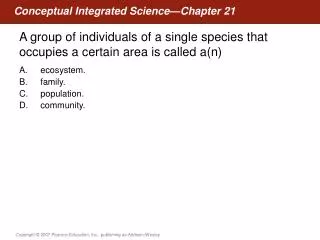
Concept 53.1: Dynamic biological processes influence population density, dispersion, and demographics. A population is a group of individuals of a single species living in the same general area Populations are described by their boundaries and size

E N D
Concept 53.1: Dynamic biological processes influence population density, dispersion, and demographics • A population is a group of individuals of a single species living in the same general area • Populations are described by their boundaries and size • Density is the number of individuals per unit area or volume • Dispersion is the pattern of spacing among individuals within the boundaries of the population
Density: A Dynamic Perspective • Usually it is impractical or impossible to count all individuals in a population so sampling techniques are used to estimate pop sizes. • Population size can be estimated by either extrapolation from small samples, an index of population size (e.g., number of nests), or the mark-recapture method
Mark-recapture method (Lincoln Index) • Scientists capture, tag, and release a random sample of individuals (s) in a population • Marked individuals are given time to mix back into the population
This calculation uses the recapture data to determine the proportion of the actual population as sampled on the first capture. Or: How much of the actual population did we catch in the first capture?
Following disaster, environmental change, disease, or over hunting, K-strategists take a long time to recover, if at all. • Monitoring of endangered or at-risk species populations is essential if they are to be preserved as it taking action to protect them. • If a population is not given time or resources to recover, it won’t.
Immigration is the influx of new individuals from other areas • Emigration is the movement of individuals out of a population Births and immigrationadd individuals toa population. Deaths and emigrationremove individualsfrom a population. Immigration Emigration
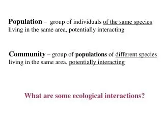
Patterns of Dispersion • Environmental and social factors influence the spacing of individuals in a population • Clumped dispersion - individuals aggregate in patches. A clumped dispersion may be influenced by resource availability and behavior
A uniform dispersion is one in which individuals are evenly distributed • It may be influenced by social interactions such as territoriality, the defense of a bounded space against other individuals
In a random dispersion, the position of each individual is independent of other individuals • It occurs in the absence of strong attractions or repulsions
Life Tables • A life table is an age-specific summary of the survival pattern of a population, & usually follows the fate of a cohort, a group of individuals of the same age • The life table of Belding’s ground squirrels reveals many things about this population • For example, it provides data on the proportions of males and females alive at each age
Survivorship Curves • A survivorship curve is a graphic way of representing the data in a life table • The survivorship curve for Belding’s ground squirrels shows a relatively constant death rate
Figure 53.5 1,000 100 Number of survivors (log scale) Females 10 Males 1 0 2 4 6 8 10 Age (years)
Survivorship curves can be classified into three general types • Type I: low death rates during early and middle life and an increase in death rates among older age groups • Type II: a constant death rate over the organism’s life span • Type III: high death rates for the young and a lower death rate for survivors • Many species are intermediate to these curves
Figure 53.6 1,000 I 100 II Number of survivors (log scale) 10 III 1 0 50 100 Percentage of maximum life span
Reproductive Rates • For species with sexual reproduction, researchers often concentrate on females in a population • A reproductive table, or fertility schedule, is an age-specific summary of the reproductive rates in a population • It describes the reproductive patterns of a population
Change in population size Immigrants entering population Emigrants leaving population Births Deaths Concept 53.2: The exponential model describes population growth in an idealized, unlimited environment Per Capita Rate of Increase • If immigration and emigration are ignored, a population’s growth rate (per capita increase) equals birth rate minus death rate
The population growth rate can be expressed mathematically as where N is the change in population size, t is the time interval, B is the number of births, and D is the number of deaths
Births and deaths can be expressed as the average number of births and deaths per individual during the specified time interval B bN D mN where b is the annual per capita birth rate, m(for mortality) is the per capita death rate, and N is population size
The per capita rate of increase (r) is given by r b m • Zero population growth (ZPG) occurs when the birth rate equals the death rate (r 0)
dN rmaxN dt Exponential Growth • Exponential population growth is population increase under idealized conditions • Under these conditions, the rate of increase is at its maximum, denoted as rmax • The equation of exponential population growth is • Exponential population growth results in a J-shaped curve
Figure 53.7 2,000 dNdt = 1.0N 1,500 dNdt = 0.5N Population size (N) 1,000 500 0 5 10 15 Number of generations
The J-shaped curve of exponential growth characterizes some rebounding populations • For example, the elephant population in Kruger National Park, South Africa, grew exponentially after hunting was banned
Figure 53.8 8,000 6,000 Elephant population 4,000 2,000 0 1900 1910 1920 1930 1940 1950 1960 1970 Year
Concept 53.3: The logistic model describes how a population grows more slowly as it nears its carrying capacity • Exponential growth cannot be sustained for long in any population • A more realistic population model limits growth by incorporating carrying capacity • Carrying capacity (K) is the maximum population size the environment can support • Carrying capacity varies with the abundance of limiting resources
(K N) dN rmax N dt K The Logistic Growth Model • In the logistic population growth model, the per capita rate of increase declines as carrying capacity is reached • The logistic model starts with the exponential model and adds an expression that reduces per capita rate of increase as N approaches K
Where is the overall population growth rate the highest & why? At N = 750, or half of K. There are enough reproducing individuals to sustain a high reproductive rate, & lots of resources still.
The logistic model of population growth produces a sigmoid (S-shaped) curve
Figure 53.9 Exponentialgrowth 2,000 dN dt = 1.0N 1,500 K = 1,500 Logistic growth 1,500 – N 1,500 dN dt ( ) Population size (N) = 1.0N 1,000 Population growthbegins slowing here. 500 0 0 5 10 15 Number of generations
The Logistic Model and Real Populations • The growth of laboratory populations of paramecia fits an S-shaped curve • These organisms are grown in a constant environment lacking predators and competitors
Figure 53.10 180 1,000 150 800 120 Number of Daphnia/50 mL Number of Paramecium/mL 600 90 400 60 200 30 0 0 0 5 10 15 0 20 40 60 80 100 120 140 160 Time (days) Time (days) (b) A Daphnia population in the lab (a) A Paramecium population in the lab
Figure 53.10b • Some populations overshoot K before settling down to a relatively stable density 180 150 120 Number of Daphnia/50 mL 90 60 30 0 0 20 40 60 80 100 120 140 160 Time (days) (b) A Daphnia population in the lab
Some populations fluctuate greatly and make it difficult to define K • Some populations show an Allee effect, in which individuals have a more difficult time surviving or reproducing if the population size is too small • The logistic model fits few real populations but is useful for estimating possible growth • Conservation biologists can use the model to estimate the critical size below which populations may become extinct
Concept 53.4: Life history traits are products of natural selection • An organism’s life history comprises the traits that affect its schedule of reproduction and survival • The age at which reproduction begins • How often the organism reproduces • How many offspring are produced during each reproductive cycle • Life history traits are evolutionary outcomes reflected in the development, physiology, and behavior of an organism
Evolution and Life History Diversity • Species that exhibit semelparity, or big-bang reproduction, reproduce once and die • Species that exhibit iteroparity, or repeated reproduction, produce offspring repeatedly • Highly variable or unpredictable environments likely favor big-bang reproduction, while dependable environments may favor repeated reproduction
“Trade-offs” and Life Histories • Organisms have finite resources, which may lead to trade-offs between survival and reproduction • For example, there is a trade-off between survival and paternal care in European kestrels
Figure 53.13 RESULTS 100 Male Female 80 60 Parents surviving the followingwinter (%) 40 20 0 Reducedbrood size Normalbrood size Enlargedbrood size
Some plants produce a large number of small seeds, ensuring that at least some of them will grow and eventually reproduce
Other types of plants produce a moderate number of large seeds that provide a large store of energy that will help seedlings become established Brazilian nuts, & nut tree
K-selection, or density-dependent selection, selects for life history traits that are sensitive to population density • r-selection, or density-independent selection, selects for life history traits that maximize reproduction • The concepts of K-selection and r-selection are oversimplifications but have stimulated alternative hypotheses of life history evolution
Exceptions: Some organisms have both r and K stage or characteristics, such as large trees, sea turtles, and many other reptiles. Some species, such as Drosophila, change strategies depending on environmental conditions.
Pest species and disease will proliferate following ecological change or a disaster as there are new opportunities for reproduction and colonization.
Concept 53.5: Many factors that regulate population growth are density dependent Population Change and Population Density • In density-independent populations, birth rate and death rate do not change with population density • In density-dependent populations, birth rates fall and death rates rise with population density