Practical Statistical Relational Learning
This overview discusses the growing field of Statistical Relational Learning (SRL) focusing on the integration of probabilistic inference, statistical learning, logical inference, and inductive logic programming. Real-world applications such as web search, medical diagnosis, and natural language processing are explored, highlighting the challenges of dealing with non-i.i.d. data and the complexities of inference in relational contexts. The presentation also outlines the benefits of SRL for predictive accuracy and domain understanding while addressing the necessary algorithms and software tools for implementation.


Practical Statistical Relational Learning
E N D
Presentation Transcript
Practical Statistical Relational Learning Pedro Domingos Dept. of Computer Science & Eng. University of Washington
Overview • Motivation • Foundational areas • Probabilistic inference • Statistical learning • Logical inference • Inductive logic programming • Putting the pieces together • Applications
Most learners assume i.i.d. data(independent and identically distributed) One type of object Objects have no relation to each other Real applications:dependent, variously distributed data Multiple types of objects Relations between objects Motivation
Examples • Web search • Information extraction • Natural language processing • Perception • Medical diagnosis • Computational biology • Social networks • Ubiquitous computing • Etc.
Costs and Benefits of SRL • Benefits • Better predictive accuracy • Better understanding of domains • Growth path for machine learning • Costs • Learning is much harder • Inference becomes a crucial issue • Greater complexity for user
Goal and Progress • Goal:Learn from non-i.i.d. data as easilyas from i.i.d. data • Progress to date • Burgeoning research area • We’re “close enough” to goal • Easy-to-use open-source software available • Lots of research questions (old and new)
Plan • We have the elements: • Probability for handling uncertainty • Logic for representing types, relations,and complex dependencies between them • Learning and inference algorithms for each • Figure out how to put them together • Tremendous leverage on a wide range of applications
Disclaimers • Not a complete survey of statisticalrelational learning • Or of foundational areas • Focus is practical, not theoretical • Assumes basic background in logic, probability and statistics, etc. • Please ask questions • Tutorial and examples available atalchemy.cs.washington.edu
Overview • Motivation • Foundational areas • Probabilistic inference • Statistical learning • Logical inference • Inductive logic programming • Putting the pieces together • Applications
Markov Networks Smoking Cancer • Undirected graphical models Asthma Cough • Potential functions defined over cliques
Markov Networks Smoking Cancer • Undirected graphical models Asthma Cough • Log-linear model: Weight of Feature i Feature i
Hammersley-Clifford Theorem If Distribution is strictly positive (P(x) > 0) And Graph encodes conditional independences Then Distribution is product of potentials over cliques of graph Inverse is also true. (“Markov network = Gibbs distribution”)
Inference in Markov Networks • Goal: Compute marginals & conditionals of • Exact inference is #P-complete • Conditioning on Markov blanket is easy: • Gibbs sampling exploits this
MCMC: Gibbs Sampling state← random truth assignment fori← 1 tonum-samples do for each variable x sample x according to P(x|neighbors(x)) state←state with new value of x P(F) ← fraction of states in which F is true
Other Inference Methods • Many variations of MCMC • Belief propagation (sum-product) • Variational approximation • Exact methods
MAP/MPE Inference • Goal: Find most likely state of world given evidence Query Evidence
MAP Inference Algorithms • Iterated conditional modes • Simulated annealing • Graph cuts • Belief propagation (max-product)
Overview • Motivation • Foundational areas • Probabilistic inference • Statistical learning • Logical inference • Inductive logic programming • Putting the pieces together • Applications
Learning Markov Networks • Learning parameters (weights) • Generatively • Discriminatively • Learning structure (features) • In this tutorial: Assume complete data(If not: EM versions of algorithms)
No. of times feature i is true in data Expected no. times feature i is true according to model Generative Weight Learning • Maximize likelihood or posterior probability • Numerical optimization (gradient or 2nd order) • No local maxima • Requires inference at each step (slow!)
Pseudo-Likelihood • Likelihood of each variable given its neighbors in the data • Does not require inference at each step • Consistent estimator • Widely used in vision, spatial statistics, etc. • But PL parameters may not work well forlong inference chains
Discriminative Weight Learning • Maximize conditional likelihood of query (y) given evidence (x) • Approximate expected counts by counts in MAP state of y given x No. of true groundings of clause i in data Expected no. true groundings according to model
Other Weight Learning Approaches • Generative: Iterative scaling • Discriminative: Max margin
Structure Learning • Start with atomic features • Greedily conjoin features to improve score • Problem: Need to reestimate weights for each new candidate • Approximation: Keep weights of previous features constant
Overview • Motivation • Foundational areas • Probabilistic inference • Statistical learning • Logical inference • Inductive logic programming • Putting the pieces together • Applications
First-Order Logic • Constants, variables, functions, predicatesE.g.: Anna, x, MotherOf(x), Friends(x, y) • Literal: Predicate or its negation • Clause: Disjunction of literals • Grounding: Replace all variables by constantsE.g.: Friends (Anna, Bob) • World (model, interpretation):Assignment of truth values to all ground predicates
Inference in First-Order Logic • Traditionally done by theorem proving(e.g.: Prolog) • Propositionalization followed by model checking turns out to be faster (often a lot) • Propositionalization:Create all ground atoms and clauses • Model checking: Satisfiability testing • Two main approaches: • Backtracking (e.g.: DPLL) • Stochastic local search (e.g.: WalkSAT)
Satisfiability • Input: Set of clauses(Convert KB to conjunctive normal form (CNF)) • Output: Truth assignment that satisfies all clauses, or failure • The paradigmatic NP-complete problem • Solution: Search • Key point:Most SAT problems are actually easy • Hard region: Narrow range of#Clauses / #Variables
Backtracking • Assign truth values by depth-first search • Assigning a variable deletes false literalsand satisfied clauses • Empty set of clauses: Success • Empty clause: Failure • Additional improvements: • Unit propagation (unit clause forces truth value) • Pure literals (same truth value everywhere)
The DPLL Algorithm if CNF is empty then returntrue else ifCNF contains an empty clause then returnfalse else ifCNF contains a pure literal xthen returnDPLL(CNF(x)) else ifCNF contains a unit clause {u} then return DPLL(CNF(u)) else choose a variable x that appears in CNF ifDPLL(CNF(x)) = truethenreturn true else returnDPLL(CNF(¬x))
Stochastic Local Search • Uses complete assignments instead of partial • Start with random state • Flip variables in unsatisfied clauses • Hill-climbing: Minimize # unsatisfied clauses • Avoid local minima: Random flips • Multiple restarts
The WalkSAT Algorithm fori← 1 to max-triesdo solution = random truth assignment for j ← 1 tomax-flipsdo if all clauses satisfied then return solution c ← random unsatisfied clause with probabilityp flip a random variable in c else flip variable in c that maximizes number of satisfied clauses return failure
Overview • Motivation • Foundational areas • Probabilistic inference • Statistical learning • Logical inference • Inductive logic programming • Putting the pieces together • Applications
Rule Induction • Given: Set of positive and negative examples of some concept • Example:(x1, x2, … , xn, y) • y:concept (Boolean) • x1, x2, … , xn:attributes (assume Boolean) • Goal: Induce a set of rules that cover all positive examples and no negative ones • Rule: xa ^ xb ^ … y (xa: Literal, i.e., xi or its negation) • Same as Horn clause: Body Head • Rule r covers example x iff x satisfies body of r • Eval(r): Accuracy, info. gain, coverage, support, etc.
Learning a Single Rule head ← y body←Ø repeat for each literal x rx← r with x added to body Eval(rx) body← body ^ best x until no x improves Eval(r) returnr
Learning a Set of Rules R ← Ø S ← examples repeat learn a single ruler R ← R U { r } S ← S − positive examples covered by r until S contains no positive examples returnR
First-Order Rule Induction • y and xiare now predicates with argumentsE.g.: y is Ancestor(x,y), xi is Parent(x,y) • Literals to add are predicates or their negations • Literal to add must include at least one variablealready appearing in rule • Adding a literal changes # groundings of ruleE.g.: Ancestor(x,z) ^Parent(z,y) Ancestor(x,y) • Eval(r) must take this into accountE.g.: Multiply by # positive groundings of rule still covered after adding literal
Overview • Motivation • Foundational areas • Probabilistic inference • Statistical learning • Logical inference • Inductive logic programming • Putting the pieces together • Applications
Plethora of Approaches • Knowledge-based model construction[Wellman et al., 1992] • Stochastic logic programs [Muggleton, 1996] • Probabilistic relational models[Friedman et al., 1999] • Relational Markov networks [Taskar et al., 2002] • Bayesian logic[Milch et al., 2005] • Markov logic[Richardson & Domingos, 2006] • And many others!
Key Dimensions • Logical languageFirst-order logic, Horn clauses, frame systems • Probabilistic languageBayes nets, Markov nets, PCFGs • Type of learning • Generative / Discriminative • Structure / Parameters • Knowledge-rich / Knowledge-poor • Type of inference • MAP / Marginal • Full grounding / Partial grounding / Lifted
Knowledge-BasedModel Construction • Logical language: Horn clauses • Probabilistic language: Bayes nets • Ground atom → Node • Head of clause → Child node • Body of clause → Parent nodes • >1 clause w/ same head → Combining function • Learning: ILP + EM • Inference: Partial grounding + Belief prop.
Stochastic Logic Programs • Logical language: Horn clauses • Probabilistic language:Probabilistic context-free grammars • Attach probabilities to clauses • .ΣProbs. of clauses w/ same head = 1 • Learning: ILP + “Failure-adjusted” EM • Inference: Do all proofs, add probs.
Probabilistic Relational Models • Logical language: Frame systems • Probabilistic language: Bayes nets • Bayes net template for each class of objects • Object’s attrs. can depend on attrs. of related objs. • Only binary relations • No dependencies of relations on relations • Learning: • Parameters: Closed form (EM if missing data) • Structure: “Tiered” Bayes net structure search • Inference: Full grounding + Belief propagation
Relational Markov Networks • Logical language: SQL queries • Probabilistic language: Markov nets • SQL queries define cliques • Potential function for each query • No uncertainty over relations • Learning: • Discriminative weight learning • No structure learning • Inference: Full grounding + Belief prop.
Bayesian Logic • Logical language: First-order semantics • Probabilistic language: Bayes nets • BLOG program specifies how to generate relational world • Parameters defined separately in Java functions • Allows unknown objects • May create Bayes nets with directed cycles • Learning: None to date • Inference: • MCMC with user-supplied proposal distribution • Partial grounding
Markov Logic • Logical language: First-order logic • Probabilistic language: Markov networks • Syntax: First-order formulas with weights • Semantics: Templates for Markov net features • Learning: • Parameters: Generative or discriminative • Structure: ILP with arbitrary clauses and MAP score • Inference: • MAP: Weighted satisfiability • Marginal: MCMC with moves proposed by SAT solver • Partial grounding + Lazy inference
Markov Logic • Most developed approach to date • Many other approaches can be viewed as special cases • Main focus of rest of this tutorial
Markov Logic: Intuition • A logical KB is a set of hard constraintson the set of possible worlds • Let’s make them soft constraints:When a world violates a formula,It becomes less probable, not impossible • Give each formula a weight(Higher weight Stronger constraint)
Markov Logic: Definition • A Markov Logic Network (MLN) is a set of pairs (F, w) where • F is a formula in first-order logic • w is a real number • Together with a set of constants,it defines a Markov network with • One node for each grounding of each predicate in the MLN • One feature for each grounding of each formula F in the MLN, with the corresponding weight w