Download
1 / 32
320 likes | 415 Vues
An Econometric Model of Sex-Specific U.S. Immigration before the Civil War Michael J. Greenwood University of Colorado at Boulder.

E N D
An Econometric Model of Sex-Specific U.S.Immigration before the Civil WarMichael J. GreenwoodUniversity of Colorado at Boulder
Donna Gabaccia: “Historical studies of international female migration scarcely exist” (1996, p. 91).A study by the United Nations (1994) indicates that little is known about women’s migration, either internal or international, and laments “the neglect of research on women’s migration” (p. xv).
Why is the sex composition of international migration important? 1. Females were less likely to be “economic migrants” than males. Economic migrants are motivated by their own economic advantages and costs. Thus, females were less likely to participate in formal labor markets upon their arrival in the U.S. 2. The child-bearing capacity of females increases the potential for growth of the second generation immigrant population.
The United States began collecting immigration data, by sex, in 1820. This is by far the earliest date that any “New World” country began systematically recording information on immigrants, by country of birth. These data are not without problems, but at least they provide a resource with which to work. Later I will discuss some of these problems, and I also will discuss my efforts to “correct” or “adjust” the data to account for the shortcomings.
Background Research on Sex-Specific MigrationRavenstein’s (1885) Seventh Law of Migration: “Females are more migratory than males.”D.S.Thomas (1938) devotes a chapter tp “sex differentials” and there she poses the following question: “What opportunities, social and economic, are offered young men and women migrants in what types of cities ? … How far is migration an adjustment to these opportunities?” (pgs. 68-69).Hatton and Williamson (1998), in their book on the era of mass migration, devote a little attention to female migration.
Donato, Katherine M. “Understanding U.S. Immigration: Why Some Countries Send Women and Others Send Men.” In Seeking Common Ground, edited by Donna Gabaccia, 159-184. Connecticut: Praeger, 1992. Donato, Katherine M. and Andrea Tyree. “Family Reunification, Health Professionals, and the Sex Composition of Immigrants to the United States.” In Sociology and Social Research 70, no. 3, edited by Marcus Freeman, 226-230. Los Angeles: University of Southern California, 1986. Greenwood, Michael J. and John M. McDowell, Legal U.S. Immigration: Influences on Gender, Age, and Skill Composition. Kalamazoo: W.E.UPJOHN Institute for Employment Research, 1999. Greenwood, Michael J., Family and Sex-Specific U.S. Immigration from Europe, 1870-1910: A Panel Data Study of Rates and Composition, Explorations in Economic History, 45 (3), Sept. 2008, 356-382.
The Model I distinguish two types of migrants: 1. Independent migrants, who presumably entered the U.S. with economic incentives primarily in mind, and 2. Accompanying migrants, who entered with an independent migrant or who followed one, but whose own economic incentives were not the primary force behind the move. Given that independent economic migrants were primarily male and accompanying migrants in immigrant family units, apart from children, were primarily female, variations in the sex composition of the total flows from the various source countries should be a function of the relative incentives for single-unit independent migration versus family-unit migration. Economic migrants should be particularly responsive to differential advantages between the U.S. and their source countries and to the relative costs of migrating, although the costs of migrating are relevant for accompanying migrants as well.
Let Mijt represent migration from country i to the United States (j) in year t: Mijt = zijt + ijt , (1) where is a vector of unknown parameters, zijt is a vector of independent variables with zijt = [xijt1, xijt2, xijt3], and ijt is random errors. Mijt may represent the migration rate from country i to the U.S. in year t or, alternatively, the female share of migrants from i to the U.S. in t. The x’s represent, respectively, variables, relating to differential economic opportunities between source countries and the U.S.(xijt1), variables relating to the costs of migrating to the U.S.(xijt2), and control variables (xijt3).
Econometric Procedures The Hausman-Taylor instrumental variable estimator (1981) is used to address the econometric problems encountered. This approach is briefly described below: mist = αi + δt + βxit + γzi + єist, i=1,…,11; t=1,…,36, (2) where mist is migration of sex s from country i in year t. Again mist could refer either a migration rate or to sex composition. The notation refers to 1820-1855. Next we partition the set of explanatory variables into two groups, paying close attention to the model’s time-invariant variables, such as distance and the dummy variable for English-speaking countries: [ xit| zi ] where xit is a Kx1 vector of variables that measures characteristics of country i in period t and zi is a Gx1 vector of time-invariant variables. (I drop the s subscript because each sex class has the same set of right-hand side variables.) In (2), β and γ are vectors of unknown parameters, єist is a random disturbance, and the vectors αi and δt are unobserved country-specific and time-specific variables, respectively.
The error terms єist are assumed to have zero mean and to be independent across countries. The model allows different cross-sectional and time-specific intercepts, and various assumptions about these are discussed in some detail in Greenwood, et al. (1996). For present purposes, only those assumptions relevant to the Hausman-Taylor approach are considered.
COMPOSITIONAL METHODOLOGY The methodology used here to examine immigrant sex composition long has been employed by economists to analyze systems of demand or expenditure equations (e.g., Leser, 1961; Pollak and Wales, 1969; Parks, 1969; and Barten, 1977) and systems of cost-share equations (e.g., Berndt and Wood, 1975). However, except for a few recent exceptions, no previous attempt to use such an approach to study the composition of migration appears to have been made. In the present context, the idea is to estimate a two-equation model, with one equation for males and the second for females, that satisfies an adding-up condition. The adding-up condition is simply that the fractions of male and female U.S. immigration from country i during year t must sum to one.
Let i represent source country, j independent variable, t year, and s sex. The share of U.S. immigration of a given sex is the dependent variable and may be expressed in the following way, where SHAREist represents the share of U.S. immigration from country i, of sex s, during year t: SHAREist = βs∑2s=1SHAREist + ∑nj=1βsjXisjt + єist, (3) where ∑2s=1 βs = 1, and ∑2s=1βsj = 0, V βj . The conditions state that the coefficients on the constant term (the share of immigration of sex s from i during t) must sum to one across the two sex equations. Moreover, if the data are otherwise the same on the right-hand side of each equation, the coefficients on each independent variable must sum to zero. Thus, if each independent variable were set at zero the sex shares would sum to one, as they must logically. Furthermore, any change in an independent variable that increases (decreases) one share must correspondingly decrease (increase) the other share, so that the shares continue to sum to one. The coefficients on the independent variables are interpreted as the percentage point change in the share of immigrants of sex s due to an incremental change in the independent variable.
Examples of earlier work using this methodology: Greenwood, Michael J. and John M. McDowell. Legal U.S. Immigration: Influences on Gender, Age, and Skill Composition. Kalamazoo: W.E.UPJOHN Institute for Employment Research, 1999. Greenwood, Michael J. “Family and Sex-Specific U.S. Immigration from Europe, 1870-1910: A Panel Data Study of Rates and Composition,” Explorations in Economic History 45 (3), Sept. 2008, 356-382. Greenwood, Michael J. “Modeling the Age and Age Composition of Late 19th Century U.S. Immigrants from Europe,” Explorations in Economic History 44, no. 2, 2007, 255-269. Greenwood, Michael J., John M. McDowell, and Donald M. Waldman. “A Model of the Skill Composition of US Immigration,” Applied Economics 28, 1996, 299-308. Greenwood, Michael J., John M. McDowell and Matt Wierman. “Source-Country Social Programs and the Age Composition of Legal US Immigrants,” Journal of Public Economics 87, no. 3-4, 2003, 739-771.
The Data As indicated earlier, the data cover 1820-1855. The data end in 1855 because the sex of U.S. immigrants is unknown for 1856-1868. The Dependent Variables The data are characterized by several shortcomings: I. The periods represented by “years” are not uniform (Davis, 1931). Prior to adopting a regular fiscal year (ending June 30) beginning in 1869, the State Department reports refer to various different “years”: (1) 1820-1832, 12 months ending September 30; (2) 1833-1843, calendar year, but the last quarter of 1832 was apparently lost in the change from one type of period to the other; (3) 1844, nine months ending September 30; (4) 1845-1849, 12 months ending September 30; (5) 1850, 15 months ending December 31; and (6) 1851-1855, calendar year. In this study, these different periods are taken into account through the econometric approach discussed above, but the two nine-month periods are multiplied by a factor of 1.33 and the 15-month period is multiplied by 0.8 so that each “year” refers to a 12-month period.
II. For certain countries and for specific years, relatively small numbers of immigrants did not report their sex. For the country and year in question, these numbers were distributed to the sexes in proportion to the known sex distribution. III. Another data issue for this period concerns the U.K. for all years. During the entire period, large numbers of immigrants (775,158 males, or 58.5 percent of all males, and 572,956 females, or 56.4 percent of all females) from the United Kingdom did not specify whether they come from England, Ireland, Scotland, or Wales. Since the United Kingdom was an extremely important source of immigrants during this period, and since Ireland must be separated form the other three, those not specified, by sex, were distributed in the same proportions as those whose origin was specified. IV. Since immigration data do not exist prior to 1820 and a five-year lag is used as an independent variable, where necessary the 1820 value is applied to earlier years.
The data set ultimately employed utilizes 12 source countries commonly used to study historical U.S. immigration: 1. Belgium, 2. Denmark, 3. France, 4. Germany, 5. Ireland, 6. Italy, 7. The Netherlands, 8. Norway, 9. Portugal, 10. Spain, 11. Sweden, and 12. the United Kingdom (England, Scotland, and Wales). However, for 1820-1855, reported data on U.S. immigration combine Norway and Sweden, so only 11 panels are available for study. These 11 countries or country groups provide 396 observations for the 36-year period under study.
Independent Variables The number of countries in the data set is critical because it imposes a degrees-of-freedom constraint on the estimated model or models. The number of independent variables included in the models may not exceed n-1, where n is the number of countries or country groups (or panels). This restriction demands that as many countries as possible be included in the analysis, because no matter which countries are included, the number is not great. The first consideration in selecting countries of origin was the availability of data on the dependent variable or variables (i.e., sex of immigrants). The second was data on the independent variables. Because a panel data technique is used in this study, annual time-series data had to be available back to 1820 (and in the case of the birth and death rates, to 1800) for each country. Certain variables (such as sex-specific population and, in some cases, per capita GDP) had to be interpolated to form a “synthetic” series. Other data (such as birth and death rates for some countries) had to be extrapolated.
The econometric modeling approach employed in this study requires a continuous time series for each time-varying variable included in the model. Other variables that do not vary over time, such as distance to the United States, are specifically treated in the econometric approach, but nonetheless must be assigned a value for each year. Consequently, any temporal “gaps” in the data must be filled for the approach to work. Measures for certain of the independent variables employed in this study are not available on an annual basis. This condition is especially true for census-based measures, such as population. Such measures were interpolated or extrapolated to yield continuous a 36 (1820-1855) year time series for each variable. Variables such as those noted above change sufficiently slowly, and a sufficient number of data points is available, that I feel that I have not done great injustice to the temporal aspect of the data. Moreover, the cross-sectional aspect of the data for years for which the gaps were filled align closely with those observations that center around census years.
Another data problem for 1820-1855 is that measures that are available or can be created for later periods are simply not available for this period. Whereas certain measures can be synthesized, for others no reasonable basis exits to generate annual observations because no data points are available for any country for any year. Thus, for 1820-1855 no information is available on sex-specific origin populations and none exists for the economically active populations. However, birth and death rates for certain countries were generated back 1800. In the sex-specific migration-rate regressions that are reported below, half the source country population is used to normalize the sex-specific flows.
Summary of Empirical Findings • Two types of variables stand out, relative per capita GDP and migration over the prior five years. Both male and female U.S. immigrants tended to come from relatively low income countries. With respect to the female regressions, these findings are interpreted to mean that relatively much migration of intact families originated in low-income countries. Respective elasticities estimated at the means are 3.90 for males and 4.52 for females (families). • The variable for the per capita GDP gap also is positive and significant. • When separate variables are introduced for origin countries and the U.S., both coefficients have the expected sign and are highly significant. Higher U.S. per capita GDP attracted immigrants, whereas higher source-country per-capita GDP discouraged U.S. immigration. • The close association between the findings for males and females is likely the result of many males and females moving together in families and thus responding to the same basic stimuli. Nevertheless, the absolute values on the respective male coefficients are greater than their counterparts for females, which is as expected since males were more likely to be economic migrants. The interaction terms are significant, which suggests that migrants from the U.K. were more responsive to wage gaps or to opportunities in the U.S., which presumably reflects their ability to transfer accumulated education and occupational skills to the U.S. labor market.
Current immigrants had a strong tendency to follow past immigrants. About 6 current male immigrants came to the U.S. per 1,000 persons who migrated over the past five years, whereas about 5 females migrated per 1,000 earlier migrants. • Other than the source-country population in the last regression for each sex, which is negative and significant, no other variable is statistically significant in any regression of Table 4. • Malthusian population pressures do not appear to have encouraged more emigration of either males or females during the early years of the nineteenth century, although they were to become more important later in the century. Higher source-country birth rates and the associated increased costs associated with larger family size do not appear to have discouraged family migration.
8. During 1820-1855, the sex composition of U.S. immigration was significantly less oriented toward females if the source countries had relatively high per capita GDP compared to the U.S. In other words, compared to males more females and thus presumably more family migrants originated in relatively low-income source countries. • Table 5 also provides estimates for per capita GDP broken down by source country and the United States. These results suggest that relative to males, females (families) were attracted by better economic opportunities in the U.S. • The interaction term between relative per capita GDP and English is negative and significant. Thus, relative to males, females from Ireland and the rest of the U.K. were less responsive to wage gaps. In the presence of the interaction term, the relative per capita GDP variable is positive and significant, which suggests that females and thus families from the rest of Europe were more responsive to economic incentives than females from the U.K.
11. Higher birth rates in source countries discouraged female migration relative to that of males, as anticipated, but current labor force pressure at entry ages (as reflected in the rate of natural increase lagged 20 years) encouraged more female migration. Thus, families relative to lone males were more influenced by population pressure during the early 19th century. 12. With the exception of the first regression of Table 5 (in which the coefficient on lagged migration is negative and significant), past migrants do not appear to have differentially influenced the current movement of females relative to males. 13. English and distance are never significant.
14. Single males moved to the U.S. from relatively high-income European source countries. During 1870-1910 single males, especially those from Ireland and Scandinavia, were relatively quite responsive to per capita GDP differences between the U.S. and their source countries (Greenwood, 2008). So why should single males have behaved differently during the early 19th century? One possibility is that England, Scotland, and Wales sent to the U.S. the most single males per million population (518.2), higher even than Ireland (507.5), and yet had the second highest per capita GDP gap favoring a European source country (-$435.31) after the Netherlands (-610.64). Of course, another possibility is that single males were drawn from the lower tail of the income distribution in their relatively high-income source countries.