Pattern Matching

Pattern Matching Pattern Matching

Outline and Reading • Strings (§11.1) • Pattern matching algorithms (§11.2) • Brute-force algorithm • Boyer-Moore algorithm • Knuth-Morris-Pratt algorithm Pattern Matching

A string is a sequence of characters Examples of strings: Java program HTML document DNA sequence Digitized image An alphabet S is the set of possible characters for a family of strings Example of alphabets: ASCII Unicode {0, 1} {A, C, G, T} Let P be a string of size m A substring P[i .. j] of P is the subsequence of P consisting of the characters with ranks between i and j A prefix of P is a substring of the type P[0 .. i] A suffix of P is a substring of the type P[i ..m -1] Given strings T (text) and P (pattern), the pattern matching problem consists of finding a substring of T equal to P Applications: Text editors Search engines Biological research Strings Pattern Matching

Brute-Force Algorithm AlgorithmBruteForceMatch(T, P) Inputtext T of size n and pattern P of size m Outputstarting index of a substring of T equal to P or -1 if no such substring exists for i  0 to n - m { test shift i of the pattern } j  0 while j < m  T[i + j]= P[j] j j +1 if j = m return i { match at i } else return -1 { no match } • The brute-force pattern matching algorithm compares the pattern P with the text T for each possible shift of P relative to T, until either • a match is found, or • all placements of the pattern have been tried • Brute-force pattern matching runs in time O(nm) • Example of worst case: • T = aaa … ah • P = aaah • may occur in images and DNA sequences • unlikely in English text Pattern Matching

Brute Force Pattern Matching

Brute Force-Complexity • Given a pattern M characters in length, and a text N characters in length... • Worst case: compares pattern to each substring of text of length M. For example, M=5. • This kind of case can occur for image data. Total number of comparisons: M (N-M+1) Worst case time complexity: O(MN) Pattern Matching

Brute Force-Complexity(cont.) • Given a pattern M characters in length, and a text N characters in length... • Best case if pattern found: Finds pattern in first M positions of text. For example, M=5. Total number of comparisons: M Best case time complexity: O(M) Pattern Matching

Brute Force-Complexity(cont.) • Given a pattern M characters in length, and a text N characters in length... • Best case if pattern not found: Always mismatch on first character. For example, M=5. Total number of comparisons: N Best case time complexity: O(N) Pattern Matching

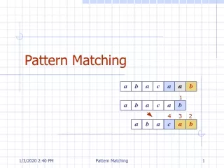
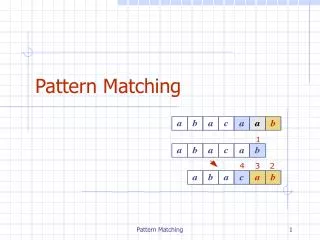
Boyer-Moore’s Algorithm (1) • The Boyer-Moore’s pattern matching algorithm is based on two heuristics Looking-glass heuristic: Compare P with a subsequence of T moving backwards Character-jump heuristic: When a mismatch occurs at T[i] = c • If P contains c, shift P to align the last occurrence of c in P with T[i] • Else, shift P to align P[0] with T[i + 1] • Example Pattern Matching

Last-Occurrence Function • Boyer-Moore’s algorithm preprocesses the pattern P and the alphabet S to build the last-occurrence function L mapping S to integers, where L(c) is defined as • the largest index i such that P[i]=c or • -1 if no such index exists • Example: • S = {a, b, c, d} • P=abacab • The last-occurrence function can be represented by an array indexed by the numeric codes of the characters • The last-occurrence function can be computed in time O(m + s), where m is the size of P and s is the size of S Pattern Matching

Case 2: 1+l j Case 1: j  1+l Boyer-Moore’s Algorithm (2) AlgorithmBoyerMooreMatch(T, P, S) L lastOccurenceFunction(P, S ) i  m-1 j  m-1 repeat if T[i]= P[j] if j =0 return i { match at i } else i  i-1 j  j-1 else { character-jump } l  L[T[i]] i  i+ m – min(j, 1 + l) j m-1 until i >n-1 return -1 { no match } Pattern Matching

Example Pattern Matching

Boyer-Moore’s algorithm runs in time O(nm + s) Example of worst case: T = aaa … a P = baaa The worst case may occur in images and DNA sequences but is unlikely in English text Boyer-Moore’s algorithm is significantly faster than the brute-force algorithm on English text Analysis Pattern Matching

KMP’s Algorithm (1) • Knuth-Morris-Pratt’s algorithm preprocesses the pattern to find matches of prefixes of the pattern with the pattern itself • The failure function F(i) is defined as the size of the largest prefix of P[0..j]that is also a suffix of P[1..j] • Knuth-Morris-Pratt’s algorithm modifies the brute-force algorithm so that if a mismatch occurs at P[j] T[i] we set j  F(j-1) Pattern Matching

KMP’s Algorithm (2) AlgorithmFailureFunction( P) i  1 j  0 F[0]  0 while i <m if P[i]= P[j] F[i ] j+1 i  i+1 j  j+1 else if j >0 j  F[j-1] else F[i ]  0 i  i+1 return F • The failure function can be represented by an array and can be computed in O(m) time Pattern Matching

KMP’s Algorithm (3) AlgorithmKMPMatch(T, P) F failureFunction(P) i  0 j  0 while i <n if T[i]= P[j] if j =m-1 return i -j{ match } else i  i+1 j  j+1 else if j >0 j  F[j-1] else i  i+1 return -1 { no match } • At each iteration of the while-loop, either • i increases by one, or • the shift amount i - j increases by at least one (observe that F(j-1)< j) • Hence, there are no more than 2n iterations of the while-loop • Thus, KMP’s algorithm runs in optimal time O(m + n) Pattern Matching

Example Pattern Matching

Pattern Matching