Download
1 / 15
150 likes | 268 Vues
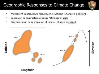
Geographic Responses to Climate Change. Movement in latitude, longitude, or elevation? (Change in position ) Expansion or contraction of range? (Change in scale ) Fragmentation or aggregation of range? (Change in shape ). time 2. time 1. Latitude. Elevation. time 1. time 2. Longitude.

E N D
Geographic Responses to Climate Change • Movement in latitude, longitude, or elevation? (Change in position) • Expansion or contraction of range? (Change in scale) • Fragmentation or aggregation of range? (Change in shape) time 2 time 1 Latitude Elevation time 1 time 2 Longitude
Key Management Questions • Abiotic: • How long will current distribution remain climatically suitable (manage for stasis)? • When and where will areas outside the current distribution become more climatically suitable (manage for change)? • Biotic: • How will biotic drivers further shape climatic response (manage for biotic-abiotic interaction)?
What we can Reliably Forecast Abiotic: Species distribution models are often used to successfully predict species’ geographic responses to climate change Biotic: Unfortunately, we still lack sufficient ecological knowledge and data to reliably forecast complex biotic-abiotic interactions Rubidge et al. (2011)
A Compromise Approach Quantitative models/forecasts Use current and future climate interpolations along with known limber pine occurrences in Rocky to model and forecast responses to climate change Expert evaluation & interpretation Scientists and managers collectively evaluate and interpret the likelihood of forecasts in light of key model assumptions and missing ecological complexity Identify management scenarios Scientists and managers collectively identify possible management scenarios that emerge from the expert evaluation and interpretation of the quantitative models and forecasts
Modeling Methods (Overview) Data Limber pine occurrence data from the vegetation inventory (polygon map) for Rocky Mountain NP Current climate data from PRISM, 1981-2010 normals (800 m); Rocky veg extent Future climate data (2035-2100, by year; time series of 30-yr normals) from PRISM-downscaled CMIP5 under both low (RCP 2.6 W/m2) and high (RCP 8.5 W/m2) emission scenarios (Thrasher et al. in prep); Rocky veg extent All monthly tmin, tmax, and precip variables transformed into 19 bioclimatic variables (see http://www.worldclim.org/bioclim) Models Weighted limber occurrences based on the % of each 800 m climate pixel covered by the species Used the weighted occurrences and current climate grids to develop a maximum entropy (Maxent) distribution model Projected current model to each future 30-yr normal (n=66) under both the RCP 2.6 and 8.5 W/m2 scenarios
Results: Model Selection Considered 6 possible parameterizations: (1) all 19 bioclimatic variables, (2) 7 annual variables, (3) 9 monthly variables, (4) 13 quarterly variables, (5) 11 temperature variables, and (6) 8 precipitation variables: Despite strong correlations among certain variables, the full (global) model parameterized using all 19 variables had the lowest AIC, and none of the other 5 models had ΔAICs ≤ 2.0 *** All subsequent results shown are for the (top performing) full 19 variable model
Results: Current Model Performance Current (1981-2010) Some over-prediction, which may reflect areas where limber pine was once present (lower elevations) Some under-prediction, but using an entropy threshold of 0.174, most under-prediction occurs in pixels where limber is < 10-15% of total area: Threshold = 0.174
Results: Future Projections A) Area may remain stable or increase until ~2055, when scenarios begin to diverge B) Elevation may increase, also until ~2055, when RCP 2.6 stabilizes C) Area may shift outside of current range until ~2055, when RCP 2.6 stabilizes D) Elevational range may shift outside of current range until ~2035-2055, when scenarios begin to diverge
Results: Future Projections Current (1981-2010) RCP 8.5 (2071-2100)
Results: Novel Future Climates MESS = Multivariate Environmental Similarity Surface Negative values = areas with novel climates for ≥ 1 variables: predictions should be treated with caution Under RCP 8.5, MESS values turn negative in 2067
Results: Novel Future Climates Variables within predicted range that are most novel, relative to present day Most Novel, RCP 8.5 Most Novel, RCP 2.6 Blue = 2035 90-100% of predicted range Red = 2100
Results: Novel Future Climates MESS, RCP 8.5 (2071-2010) Most Novel, RCP 8.5 (2071-2100)
Summary / Interpretation of Results • Limber pine can likely exist at lower populations in Rocky because: • It has the widest elevational range of any tree species in Colorado, and • The current model predicts suitable yet unoccupied climates at lower elevations • It is probably absent at lower elevations because it is being outcompeted by more shade-tolerant conifers • Expanding the lower elevational limit might help buffer the upslope distributional shift and alpine invasion predicted under both low (RCP 2.6) and high (RCP 8.5) emissions scenarios. Can we do an experiment to test whether/how 1 or 2-yr old limber seedlings survive at new low elevation sites?
Summary / Interpretation of Results • Limber pine in Rocky can likely colonize upslope because: • Alpine soils are suitable (SSURGO), and • Bioclimates at higher elevations will become suitable • However, model predictions do not explicitly consider wind and snow depth, which affect bud freeze and winter survival • Nonetheless, the upslope movement is likely possible because • Wind and snow depth will be to varying degrees correlated with other bioclimate variables included in the model, and • Drift and wind structures could be used to selectively promote initial growth/expansion
Summary / Interpretation of Results • Considering the current and 2035 model predictions, it appears that limber is already in the process of moving upslope. • Is there any data to test this, or can it be confirmed / discounted based on expert knowledge? • Should we do a survey? • If predictions are being realized, what factors characterize the colonization areas? Particular soils, slope, aspect, microrefugia, proximity to other limber stands, proximity to pine beetle outbreaks, etc? • If predictions are not being realized, can we do an experiment to determine why not?