Download
1 / 25
250 likes | 691 Vues
Price elasticity of demand. Often in economics we look at how the value of one variable changes when another variable changes. The concept called elasticity is a summary statement about those changes. . Elasticity .

E N D
Price elasticity of demand Often in economics we look at how the value of one variable changes when another variable changes. The concept called elasticity is a summary statement about those changes.
Elasticity The law of demand or the law of supply is a statement about the direction of change of the quantity demanded, or supplied, respectively, when there is a price change. The concept of elasticity adds to these concepts by indicating the magnitude of the change in quantity, given the price change. The magnitude of the change is reported in percentage terms.
own price elasticity of demand Ed = (% change in Q)/(% change in P) As an example, if Ed = -2 we say for every 1 % change in the price of the good the quantity demand changed in the opposite direction by 2 %.
absolute value You may recall a function in math called the absolute value. Basically this function makes negative values positive and leaves positive values positive. In the notes I will write abs( ) to mean take the absolute value. The own price elasticity of demand is a negative number, so we will take the absolute value to describe some concepts about it.
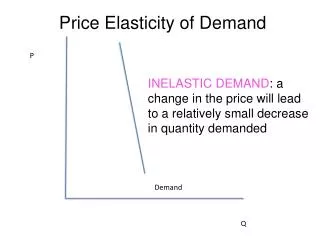
Elasticity can have three basic values If abs(Ed) > 1 we say demand is elastic. This means the % change in the Qd is greater than the % change in price. If abs(Ed) = 1 we say demand is unit elastic. This means the % change in the Qd is equal to the % change in price. If abs(Ed) < 1 we say demand is inelastic. This means the % change in the Qd is less than the % change in price.
Elasticity again P In the upper left of the demand curve the % change in the Qd is greater than the % change in the P and thus the Ed > 1 . P1 P2 Q Q1 Q2 Without a real formal proof of the above statement, we can see the % change in Qd is about 100 % and the % change in P is less than 100 %. Demand is elastic here.
Elasticity has several ranges of values P In the lower right of the demand curve the % change in the Qd is less than the % change in the P and thus the Ed < 1. P1 P2 Q Q1 Q2 Without a real formal proof of the above statement, we can see the % change in Qd is less than 100 % and the % change in P is about 100 %. Demand is inelastic here.
Elasticity has several ranges of values P In the middle of the demand curve the % change in the Qd is equal to the % change in the P and thus the Ed = 1. P1 P2 Q Q1 Q2 Without a real formal proof of the above statement, we can see the % change in Qd is about equal to the % change in P. Demand is unit elastic here.
Calculation point slope method If we know the slope of the demand curve the elasticity at a point is found by using the Q and P value of the point and the slope in the following way: (P/Q)(1/slope). Example say the slope here is -1. The elasticity is (11/10)(1/-1) = -1.1 When we take absolute value we get 1.1. Elastic in this case. P 11 10 Q
Own price elasticity and total revenue changes Total revenue (TR) is price times quantity. Along the demand curve P and Q move in opposite directions. Knowledge of Ed assists in knowing how TR will change.
Elasticity and total revenue relationship When we look at the collection of consumers in the market, at this time in our study we assume each consumer pays the same price per unit for the product. Also at this time in our study the total expenditure of the consumers in the market would equal the total revenue (TR) to the sellers. So, here we look at the whole demand side of the market in general.
Elasticity and total revenue relationship P TR in the market is equal to the price in the market multiplied by the quantity traded in the market. In this diagram TR equals the area of the rectangle made by P1, Q1 and P1 Q Q1 the horizontal and vertical axes. We know from math that the area of a rectangle is base times height and thus here that means P times Q.
Elasticity and total revenue relationship We will want to look at the change in values of a variable and in order to do so we want to have a consistent measure of change. In this regard let’s say the change in a variable is the later value minus the earlier value. Thus if the price should change from P1 to P2, then the change in price is P2 - P1, or similarly if the TR should change the change in TR is TR2 - TR1.
Elasticity and total revenue relationship P Now in this graph when the price is P1 the TR = a + b(adding areas) and if the price is P2 the TR = b + c. The change in TR if the price should fall P1 P2 a b c Q Q1 Q2 from P1 to P2 is (b + c) - (a + b) = c - a. Similarly, if the price should rise from P2 to P1 the change in TR is a - c. I will focus on price declines next.
Elasticity and total revenue relationship P Since the change in TR is c - a, the value of the change will depend on whether c is bigger or smaller, or even equal to, a. In this diagram we see c > a and thus the change in TR > 0. P1 P2 a b c Q Q1 Q2 This means that as the price falls, TR rises. I think you will recall that in the upper left of the demand the demand is price elastic. Thus if the price falls in the elastic range of demand TR rises.
Elasticity and TR You will note on the previous screen that I had c - a. In the graph c is indicating the change in TR because we are selling more units. The area a is indicating the change in TR when there is a price change. We have to bring the two together to get the change in TR. Thus a lower price has a good and a bad. Good - sell more units. Bad - sell at lower price.
Elasticity and total revenue relationship P Now in this graph when the price is P1 the TR = a + b(adding areas) and if the price is P2 the TR = b + c. In this diagram we see c < a and thus the change in TR < 0. P1 P2 a b c Q Q1 Q2 I think you will recall that in the lower right of the demand the demand is price inelastic. Thus if the price falls in the inelastic range of demand TR falls.
Elasticity and total revenue relationship P Now in this graph when the price is P1 the TR = a + b(adding areas) and if the price is P2 the TR = b + c. In this diagram we see c = a and thus the change in TR = 0. P1 P2 a b c Q Q1 Q2 I think you will recall that in the middle of the demand the demand is unit elastic. Thus if the price falls in the unit elastic range of demand TR does not change.
Elasticity and TR P When the price falls the quantity demanded always rises. As the quantity demanded rises (because of the price change) the TR is first rising in the elastic range, levels off when demand is unit elastic and TR falls in the inelastic range. D Q TR Q
Marginal revenue Marginal revenue is defined as the change in total revenue as the number of units cold changes. In the demand graph we have seen that in order to sell more the price has to be lowered. So, there is a relationship between elasticity and marginal revenue. If price falls and demand is elastic we know TR rises so MR is positive. If Price falls and demand is inelastic we know TR falls and so MR is negative. If price fall and demand is unit elastic we know TR does not change.
Other demand elasticities There are other elasticities besides the own price elasticity of demand. Let’s see a few here.
demand shifters We saw that things like taste and preference, price of other goods, income and the number of buyers shift the demand curve if they change. How much do they shift the demand curve? We use other elasticity concepts as an indication of how much the curve will shift given a change in one of these factors.
cross price elasticity of demand Edxy = % change in Qdx / % change in Py. The bigger the value the more the demand shifts. If the value is negative we have complements and if positive we have substitutes. If the absolute value is between 0 and 1 the cross elasticity is inelastic, if = 1 unit elastic and if greater than 1 elastic.
income elasticity of demand Edxm = % change in Qdx / % change in M. The bigger the value the more the demand shifts. If the value is negative we have an inferior good and if positive we have a normal good. If the absolute value is between 0 and 1 the income elasticity is inelastic, if = 1, unit elastic, and if greater than 1, elastic.
Elasticity of supply The elasticity of supply is used to indicate the percentage change in the quantity supplied given a percentage change in price. The elasticity of supply is calculated in a manner similar to the other elasticities we have seen and has a similar interpretation in terms of the range of values the elasticity might take, i.e. elastic, inelastic and unit elastic.