Download
1 / 37
370 likes | 542 Vues
Modelling and Simulation of Complex Systems COST 286, Wroclaw 17-18 Sept 2003. Christos CHRISTOPOULOS Professor of Electrical Engineering Electromagnetics Research Group (ERG) School of Electrical and Electronic Engineering University of Nottingham, Nottingham, NG7 2RD, UK

E N D
Modelling and Simulation of Complex SystemsCOST 286, Wroclaw 17-18 Sept 2003 Christos CHRISTOPOULOS Professor of Electrical Engineering Electromagnetics Research Group (ERG) School of Electrical and Electronic Engineering University of Nottingham, Nottingham, NG7 2RD, UK christos.christopoulos@nottingham.ac.uk
Outline: • Profile of ERG • Modelling and simulation of complex systems at Nottingham • Coupling models for emission and susceptibility in multi-wire transmission systems • Whole System Modelling • Coupled physical domain models • Outlook
Profile of ERG: • Five full-time academic members and an experimental officer • Ten research associates • Ten research students • Five visiting scholars
22 funded research projects • Total current external funding £2,850,000 • Current areas of interest: • Fundamental development of CEM methods • Multi-scale modelling • Semi-analytical modelling techniques • Modelling and simulation for EMC/SI • Modelling and Simulation in Opto-electronics and Photonics • Coupled physical domain models • Fast transients and fault detection
Modelling and simulation of complex systems at Nottingham: • Coupling models for emission and susceptibility in multi-wire transmission systems • Whole system modelling • Coupled physical domain models
Coupling models for emission and susceptibility in multi-wire transmission systems The main effort in this area is to devise algorithms which can be embedded into general EM field solvers to describe complex wiring systems such as wire looms. This is typical of a multi-scale problem where the details of a wire loom are just too fine to be described in the conventional way as part of the modelling mesh. The solution is self consistent and hence accurate within the limitations of the numerical model. Issues addressed are, arbitrary placement, field-to-wire coupling and cross-talk, both for emission and susceptibility.
There are four approaches to this problem: • Separated solution (not self-consistent but simple to apply) • Conventional Holland model for single wire (quasi-static approximation) • Multi-wire models based on the quasi-static formulation of Holland • Multi-wire models based on the a modal expansion technique (MET)
y=d y=0 y z x Field-to-wire coupling:
DEVELOPMENT OF A WIRE INTERFACE BETWEEN TLM NODES (quasi-static approximation according to Holland) Consider a wire directed along the z-direction. From Maxwell’s curl equations in cylindrical coordinates: Integrating this equation from the wire radius ‘a’ to some radius , and using the approximation that near the wire static conditions apply ie
where I is the conductor current and Q is the charge per unit length, gives after some manipulation: In this expression Ld and Cd are the wire inductance and capacitance with respect to some reference return conductor at a radius . We will discuss latter what this should be. Ez( ) is the field at this radius. This expression tells us how the electric field and the conductor current and charge are related.
4 2 7 3 8 10 9 1 5 Let us place a wire directed along the z-axis! Port 10 of the (x,y,z) node couples with the wire 12 12 4 2 7 3 11 11 8 6 6 10 9 1 5 Port 6 of the (x+Dl,y,z) node couples with the wire y x z
Our task now is to enforce the conditions described by the field-wire equation into the TLM mesh KVL in each loop represents previous equation y reference x z
Stub round trip time The coupling to the field nodes is through ports 1 and 2 above.
A segment of a multi-wire bundle directed along the z-direction is shown through the centre of a node of length Dz U and V indicate incident and reflected voltages n-conductors ‘reference’ To next node at lower coordinate To next node at higher coordinate + Coupling to the field at the centre of the reference Dz Propagation delay along Dz is Dt
The treatment is very similar to that of the previous case (single wire through a node) but instead of voltage pulses we have voltage pulse vectors, and instead of impedances we have impedance matrices. In what follows, if n is the number of conductors in the bundle: Bundle capacitance and inductance per unit length, nxn matrices. Bundle impedance matrix, nxn. Stub parameters, nxn matrices. Incident and reflected voltage column vectors, n-elements.
Further Reading: ‘A fully integrated multi-conductor model for TLM’, IEEE Trans on MTT, 46, 1998, pp 2431-2437, J Wlodarczyk, V Trenkic, R A Scaramuzza, C Christopoulos ‘Multi-scale modelling in time-domain electromagnetics’, Int Journal of Electronics and Communications (AEU), 57, 2003, pp 100-110 , C. Christopoulos
Modal Expansion Technique (MET) : the Holland and Simpson type of approach is inaccurate because there is insufficient information contained in the static solution for a wire. The general response of a wire to an incident field is to generate a scattered field which in combination with the incident field is rich in modal information: The static solution is but the first term in this expansion-but there is much more information available!
At the edges of a node containing a wire, we can calculate the impedance seen by each field mode. Without significant loss in accuracy we can use the small argument expansions for the Bessel functions to get: D is half the nodal spacing, and a is the wire radius
It is now possible to proceed in two different ways: • Construct an equivalent circuits to ensure that the modal components of incident voltages encountering a node containing a wire see the correct impedance as calculated earlier • Treat the reflection of signals as a signal processing task and by-pass the construction of the equivalent circuit. • Either method can be applied. The advantage of the circuit approach is that it keeps with the philosophy of TLM and the fact that such a circuit can be constructed is a guarantee of stability
Electric Field, V/m MET analytic between node centre node Frequency ratio, f/fmax Example: Comparison of MET with analytical results and other wire models (mesh resolution 50mm, wore radius 5mm). The problem is of an incident field scattered by the wire. The total field is shown 100mm in front of the wire.
Further reading: ‘An accurate 3D model for thin wire simulations’, IEEE Trans on EMC, 45, 2003, pp 207-217, P Sewell, Y K Choong, C Christopoulos
Whole system modelling • Intermediate models (in collaboration with the University of York) • Full-field models • Full-field models with embedded algorithms (DFI)
aperture 12 cm 30 cm 30 cm Enclosure Geometry
Further Reading:“Shielding effectiveness of a rectangular enclosure with a rectangular aperture”M P Robinson et al, Electronics Letters, 15 Aug 1996, 32(17), pp 1559-1560“An evaluation of the shielding effectiveness of cabinets”J D Turner et al, 12th Int. Zurich EMC Symp., Feb. 18-20 1997, pp 229-234“A comparison of the analytical, numerical and approximate models for shielding effectiveness with measurements”P Sewell et al, IEE Proc. Sci. Meas. Technol., 145(2), Mar. 1998, pp 61-66
Further Reading:see session TU2B, ‘Numerical Methods for Challenging Problems’, 1998 IEEE EMC Symp., 24-28 Aug 1998, Denver Co., USAin particular paper:“Application of the TLM method to equipment shielding problems”, C. Christopoulos, ibid, pp 188-193
x,y,z x+1,y,z Figure Fine feature at the interface of neighboring nodes V11 V10 V5 V4 x,y,z x+1,y,z Figure Schematic showing part of the usual connection process between two adjacent TLM nodes How connection algorithm is modified to account for perforated wall a) - scattering, Where Viare twelve incident voltages, Vrare twelve reflected voltages, k is time-step, [S] is the scattering matrix, [C ] is the connection matrix. b) - connection, Simple swapping of the voltages New scattering connection of the voltages R and T are frequency-dependent
Outline of the Digital Filter Interface (DFI) Scattering coefficients: Analytical solution Scattering coefficients: Data from measurements Scattering coefficients: Numerical simulation or or Frequency domain Extraction of zeros and poles from the Pade-approximation Sij(z) Bilinear z-transform “Discrete time” domain
DIGITAL FILTER INTERFACE: FILTER IMPLEMENTATION B0 + + 1’ z-1 B’ Vincident + Vreflected + Figure Signal-flow graph of the equivalent digital filter Figure The boundary with the digital filter between two cells • The advantages of this approach are: • accuracy • a small number of parameters after pre-processing • possibility of extracting parameters from raw frequency-domain data • low computational costs compared to the standard models • mesh resolution determined by global considerations and not by the fine features
4mm 10mm sensor 292 mm 146 mm 28 mm 20 mm Figure Pattern of the perforated wall: triangular lattice. 78 mm 20 mm 40 mm 212 mm 40 mm TEST ENCLOSURE WITH PERFORATED WALL Transmission and reflection coefficients of the perforations [C.C. Chen. IEEE MTT-21,pp.1-6]: (A, B are geometrical characteristics of the screen, l is the thickness): Figure Enclosure with perforated wall. Two TLM meshes of different scales were used in numerical models of the enclosure: a) 66x66x28 cells of the size X = 9.73mm ; b) 33x33x14 cells of the size X =19.5 mm.
Figure Measurement and simulation results for the shielding effectiveness of the enclosure. COMPARISONS 3D-TLM SIMULATION AND EXPERIMENT RESULTS
Further reading: ‘The use of digital filtering techniques for the simulation of fine features in EMC problems solved in the time domain’, IEEE Trans on EMC, 45, 2003, pp 238-244, J Paul, V Podlozny, C Christopoulos
Coupled physical domain models • Sophisticated models of materials to allow combined EM/thermal calculations for dossimetry • Combined electronic/photonic models • Further reading: • ‘Generalised material models in TLM-Part 1:Materials with frequency dependent properties’, IEEE Trans on AP, 47, 1999, pp1528-1534; Part 2: Materials with anisotropic properties, ibid. 47, pp 1535-1542; Part 3: Materials with non-linear properties, ibid. 50, 2002, pp 997-1004, J D Paul, C Christopoulos, D W P Thomas
Outlook: • Better models for multi-scale problems • General integrated multi-wire models arbitrarily placed in a 3D mesh • Macro-models for frequently occurring features • Direct radiation from chips • Statistical aspects of EMI source and system configuration