Download
1 / 46
460 likes | 533 Vues
Key Word: Path Calibration. High Resolution Finite Fault Inversions for M>4.8 Earthquakes in the 2012 Brawley Swarm. Shengji Wei. Acknowledgement Don Helmberger (Caltech) Rob Graves and Ken Hudnut , (USGS) Susan Owen, Eric Fielding, Zhen Liu, Jay Parker and Andrea Donnellan (JPL).

E N D
Key Word: Path Calibration High Resolution Finite Fault Inversions for M>4.8 Earthquakes in the 2012 Brawley Swarm ShengjiWei Acknowledgement Don Helmberger (Caltech) Rob Graves and Ken Hudnut, (USGS) Susan Owen, Eric Fielding, Zhen Liu, Jay Parker and Andrea Donnellan (JPL)
Outline • Overview of the 2012 Brawley swarm • Path calibration from the Mw3.9 earthquake • Waveform inversion of the M>5 events up to 3Hz • Complementary slip distribution (triggering?) • Two shallow (depth ~ 2.0km) normal earthquakes: seismological, field observation and geodetic evidence • Joint inversion for the Mw4.9 normal earthquake • Aseismic and seismic slip on the normal fault • Conclusion
Overview Wei, et. al., 2013, GRL Seismicity from Hauksson et. al. 2013, SRL
Finite Fault Inversion Method We need a layered crustal model to calculate synthetic seismogram: A simulated annealing algorithm is used to simultaneously invert for the: slip amplitude, slip direction, rise time, rupture velocity Jiet. al., 2002a, BSSA We need 1D velocity model(s) if not 3D. Chi-Chi Earthquake
3D velocity model: CVM-H-11.9.0 Basin Thickness 2D horizontal cuts Earthquake depth: ~5km D=2.5km D=4.5km D=0.5km
Path Calibration using the Mw3.9 Event Vs = (Vp – 1.36)/1.16 for Vp < 4.0km/s Brocher, 2005, BSSA frequency band: 0.05 ~ 3 Hz
Sensitivity for velocity structure Model used to generate synthetic data: PCM PCM CVM4.0 CVMH_11.9.0
Point source double-couple moment tenor Waveform inversions at different frequency bands show similar results
Grid Search result using the M4.6 event Only a small window fits all components Tan. Ver. Rad. Vp_top 1Hz Velocity Station: 11369
UAVSAR data (RPI 265) and field observation Static only inversion Poster: 058 (by Ken Hudnut)
Strong motion waveform fits and prediction Data used (10s~4Hz)
Vr=1.25km/s Rupture Velocity Vr=1.75km/s Vr=2.25km/s Enough redundancy is set for the rise time
Vertical Deformation Measured by Leveling Before the swarm With the swarm
Conclusion • Path calibrations are needed for high resolution finite fault inversions. • M5.3 and M5.4 events have complementary slip distribution. • The shallow M4.9 normal earthquake has a centroid depth of ~2.0km and average rupture speed is 1.75km/s. • The aseismic and seismic slip for the M4.9 normal earthquake is complementary to each other.
Strike-Slip Faulting Hauksson et. al., 2013
Depth Phases pP Time table (PCM) Dep(km) Tp(s) Ts(s) 1.00 0.469 1.609 1.50 0.646 2.008 2.00 0.800 2.314 2.50 0.935 2.562 3.01 1.059 2.779 3.51 1.176 2.981 4.01 1.285 3.169 4.51 1.387 3.346 5.01 1.484 3.512 7.54 1.945 4.305 9.74 2.334 4.974 11.9 2.712 5.625
Looking Angle Direction Cosine U-D N-S E-W
North Brawley Operations • North Brawley: 49.9 MW net - 2009 • Currently operating at approximately 33 net MW • Annual Volume of Fluid Produced: 57,000 million gallons • Annual Volume of Fluid Injected: 53,000 million gallons • 19 injection wells • Average well depth 3900 feet • Injection all < 3500 feet • Deepest injection at ~6000 feet • Salinity: Average 40,000 ppm (TDS) • Binary Fluid Injection Temperature: 150F • Temperature in the Injection Zone : 150 to 410F • Injection Rate: Average is 525 gpm • Injection Pressure: Average is 330 psig • Not allowed to exceed fracture gradient at shallowest perforations
North Brawley Seismic Array and Wells Production wells:RED Injection wells:BLUE Seismic Stations: YELLOW
Is there large amount of aseismic slip? static offset is pure prediction
11369 waveform prediction for the shallow normal earthquake (M4.6)